Logit Employment Binary Allocation Lalonde Training Example
Source:vignettes/ffv_opt_sobin_rkone_allfc_training_logit.Rmd
ffv_opt_sobin_rkone_allfc_training_logit.RmdExample using the Lalonde Training Dataset. Estimate A and alpha from logit regression. Solve for optimal binary allocation queues. There are 722 observations, 297 in the treatment group, 425 in the control group.
Objective One:
estimate a logit regression using the Lalonde (1986) dataset. Include age, education, and race as controls.
Generate and Analyze \(A_i\) and \(\alpha_i\)
- Generate and show how to generate \(A_i\) and \(\alpha_i\) in the binary allocation Space
- What is the correlation between \(A\) and \(\alpha\)
- What is the relationship between \(x\) and \(A\) and \(\alpha\), when there is one x covariate, when there are multiple?
Solve for Optimal Allocations
Uses the binary allocation function as well as the planner iterator to solve for optimal binary targeting queue. These queue tell the planner, given the planner’s preferences, who should optimally receive allocations.
Set Up
Get Data
spt_img_save <- '../_img/'
spt_img_save_draft <- 'C:/Users/fan/Documents/Dropbox (UH-ECON)/repos/HgtOptiAlloDraft/_img/'
# Dataset
data(df_opt_lalonde_training)

# Add a binary variable for if there are wage in year 1975
dft <- df_opt_lalonde_training %>%
  mutate(re75_zero = case_when(re75 == 0 ~ 1, re75 != 0 ~ 0))

# dft stands for dataframe training
dft <- dft %>% mutate(id = X) %>%
           select(-X) %>%
           select(id, everything()) %>%
           mutate(emp78 =
                    case_when(re78 <= 0 ~ 0,
                              TRUE ~ 1)) %>%
           mutate(emp75 =
                    case_when(re75 <= 0 ~ 0,
                              TRUE ~ 1))

# Generate combine black + hispanic status
# 0 = white, 1 = black, 2 = hispanics
dft <- dft %>%
    mutate(race =
             case_when(black == 1 ~ 1,
                       hisp == 1 ~ 2,
                       TRUE ~ 0))

dft <- dft %>%
    mutate(age_m2 =
             case_when(age <= 23 ~ 1,
                       age >  23~ 2)) %>%
    mutate(age_m3 =
             case_when(age <= 20 ~ 1,
                       age > 20 & age <= 26 ~ 2,
                       age > 26 ~ 3))

dft$trt <- factor(dft$trt, levels = c(0,1), labels = c("ntran", "train"))

summary(dft)
## id trt age educ black
## Min. : 1.0 ntran:425 Min. :17.00 Min. : 3.00 Min. :0.0000
## 1st Qu.: 181.2 train:297 1st Qu.:19.00 1st Qu.: 9.00 1st Qu.:1.0000
## Median : 361.5 Median :23.00 Median :10.00 Median :1.0000
## Mean : 854.4 Mean :24.52 Mean :10.27 Mean :0.8006
## 3rd Qu.:1458.5 3rd Qu.:27.00 3rd Qu.:11.00 3rd Qu.:1.0000
## Max. :4110.0 Max. :55.00 Max. :16.00 Max. :1.0000
##
## hisp marr nodeg re74
## Min. :0.0000 Min. :0.000 Min. :0.0000 Min. : 0.0
## 1st Qu.:0.0000 1st Qu.:0.000 1st Qu.:1.0000 1st Qu.: 0.0
## Median :0.0000 Median :0.000 Median :1.0000 Median : 0.0
## Mean :0.1053 Mean :0.162 Mean :0.7798 Mean : 2102.3
## 3rd Qu.:0.0000 3rd Qu.:0.000 3rd Qu.:1.0000 3rd Qu.: 824.4
## Max. :1.0000 Max. :1.000 Max. :1.0000 Max. :39570.7
## NA's :277
## re75 re78 re75_zero emp78
## Min. : 0.0 Min. : 0 Min. :0.0000 Min. :0.0000
## 1st Qu.: 0.0 1st Qu.: 0 1st Qu.:0.0000 1st Qu.:0.0000
## Median : 936.3 Median : 3952 Median :0.0000 Median :1.0000
## Mean : 3042.9 Mean : 5455 Mean :0.4003 Mean :0.7285
## 3rd Qu.: 3993.2 3rd Qu.: 8772 3rd Qu.:1.0000 3rd Qu.:1.0000
## Max. :37431.7 Max. :60308 Max. :1.0000 Max. :1.0000
##
## emp75 race age_m2 age_m3
## Min. :0.0000 Min. :0.000 Min. :1.000 Min. :1.000
## 1st Qu.:0.0000 1st Qu.:1.000 1st Qu.:1.000 1st Qu.:1.000
## Median :1.0000 Median :1.000 Median :1.000 Median :2.000
## Mean :0.5997 Mean :1.011 Mean :1.486 Mean :1.965
## 3rd Qu.:1.0000 3rd Qu.:1.000 3rd Qu.:2.000 3rd Qu.:3.000
## Max. :1.0000 Max. :2.000 Max. :2.000 Max. :3.000
##
# X-variables to use on RHS
ls_st_xs <- c('age', 'educ',
              'black','hisp','marr', 'nodeg')
svr_binary <- 'trt'
svr_binary_lb0 <- 'ntran'
svr_binary_lb1 <- 'train'
svr_outcome <- 'emp78'
sdt_name <- 'NSW Lalonde Training'
Logit Regression
Prediction with Observed Binary Input
Logit regression with a continuous variable and a binary variable. Predict outcome with observed continuous variable as well as observed binary input variable.
# Regress No bivariate
rs_logit <- glm(as.formula(paste(svr_outcome,
                                 "~", paste(ls_st_xs, collapse="+")))
                ,data = dft, family = "binomial")
summary(rs_logit)
##
## Call:
## glm(formula = as.formula(paste(svr_outcome, "~", paste(ls_st_xs,
## collapse = "+"))), family = "binomial", data = dft)
##
## Deviance Residuals:
## Min 1Q Median 3Q Max
## -2.2075 -1.4253 0.7851 0.8571 1.1189
##
## Coefficients:
## Estimate Std. Error z value Pr(>|z|)
## (Intercept) 2.90493 0.99594 2.917 0.00354 **
## age -0.01870 0.01295 -1.445 0.14855
## educ -0.02754 0.06653 -0.414 0.67896
## black -1.16273 0.38941 -2.986 0.00283 **
## hisp -0.12130 0.51185 -0.237 0.81267
## marr 0.30300 0.24551 1.234 0.21714
## nodeg -0.29036 0.27833 -1.043 0.29684
## ---
## Signif. codes: 0 '***' 0.001 '**' 0.01 '*' 0.05 '.' 0.1 ' ' 1
##
## (Dispersion parameter for binomial family taken to be 1)
##
## Null deviance: 844.33 on 721 degrees of freedom
## Residual deviance: 818.46 on 715 degrees of freedom
## AIC: 832.46
##
## Number of Fisher Scoring iterations: 4
dft$p_mpg <- predict(rs_logit, newdata = dft, type = "response")

# Regress with bivariate
# rs_logit_bi <- glm(as.formula(paste(svr_outcome,
#                                     "~ factor(", svr_binary,") + ",
#                                     paste(ls_st_xs, collapse="+")))
#                    , data = dft, family = "binomial")
rs_logit_bi <- glm(emp78 ~
                     age + I(age^2) + factor(age_m2)
                   + educ + I(educ^2) +
                   + educ + black + hisp + marr + nodeg
                   + factor(re75_zero) +
                   + factor(trt)
                   + factor(age_m2)*factor(trt)
                   , data = dft, family = "binomial")
summary(rs_logit_bi)
##
## Call:
## glm(formula = emp78 ~ age + I(age^2) + factor(age_m2) + educ +
## I(educ^2) + +educ + black + hisp + marr + nodeg + factor(re75_zero) +
## +factor(trt) + factor(age_m2) * factor(trt), family = "binomial",
## data = dft)
##
## Deviance Residuals:
## Min 1Q Median 3Q Max
## -2.3314 -1.2633 0.6740 0.8411 1.1460
##
## Coefficients:
## Estimate Std. Error z value Pr(>|z|)
## (Intercept) 5.751196 2.506147 2.295 0.02174 *
## age -0.112096 0.122321 -0.916 0.35945
## I(age^2) 0.001796 0.001853 0.969 0.33246
## factor(age_m2)2 -0.171237 0.379441 -0.451 0.65178
## educ -0.464884 0.427172 -1.088 0.27647
## I(educ^2) 0.024604 0.023252 1.058 0.29000
## black -1.129512 0.392581 -2.877 0.00401 **
## hisp -0.115414 0.515851 -0.224 0.82296
## marr 0.333527 0.250470 1.332 0.18299
## nodeg -0.050435 0.350041 -0.144 0.88543
## factor(re75_zero)1 -0.387920 0.177229 -2.189 0.02861 *
## factor(trt)train 0.413494 0.262722 1.574 0.11551
## factor(age_m2)2:factor(trt)train -0.074633 0.359556 -0.208 0.83557
## ---
## Signif. codes: 0 '***' 0.001 '**' 0.01 '*' 0.05 '.' 0.1 ' ' 1
##
## (Dispersion parameter for binomial family taken to be 1)
##
## Null deviance: 844.33 on 721 degrees of freedom
## Residual deviance: 803.66 on 709 degrees of freedom
## AIC: 829.66
##
## Number of Fisher Scoring iterations: 4
# Predcit Using Regresion Data
dft$p_mpg_hp <- predict(rs_logit_bi, newdata = dft, type = "response")

# Predicted Probabilities am on mgp with or without hp binary
scatter <- ggplot(dft, aes(x=p_mpg_hp, y=p_mpg)) +
      geom_point(size=1) +
      # geom_smooth(method=lm) + # Trend line
      geom_abline(intercept = 0, slope = 1) + # 45 degree line
      labs(title = paste0('Predicted Probabilities ', svr_outcome, ' on ', ls_st_xs, ' with or without hp binary'),
           x = paste0('prediction with ', ls_st_xs, ' and binary ', svr_binary, ' indicator, 1 is high'),
           y = paste0('prediction with only ', ls_st_xs),
           caption = paste0(sdt_name, ' simulated prediction')) +
      theme_bw()
print(scatter)
Prediction with Binary set to 0 and 1
Now generate two predictions. One set where binary input is equal to 0, and another where the binary inputs are equal to 1. Ignore whether in data binary input is equal to 0 or 1. Use the same regression results as what was just derived.
Note that given the example here, the probability changes a lot when we
# Previous regression results
summary(rs_logit_bi)
##
## Call:
## glm(formula = emp78 ~ age + I(age^2) + factor(age_m2) + educ +
## I(educ^2) + +educ + black + hisp + marr + nodeg + factor(re75_zero) +
## +factor(trt) + factor(age_m2) * factor(trt), family = "binomial",
## data = dft)
##
## Deviance Residuals:
## Min 1Q Median 3Q Max
## -2.3314 -1.2633 0.6740 0.8411 1.1460
##
## Coefficients:
## Estimate Std. Error z value Pr(>|z|)
## (Intercept) 5.751196 2.506147 2.295 0.02174 *
## age -0.112096 0.122321 -0.916 0.35945
## I(age^2) 0.001796 0.001853 0.969 0.33246
## factor(age_m2)2 -0.171237 0.379441 -0.451 0.65178
## educ -0.464884 0.427172 -1.088 0.27647
## I(educ^2) 0.024604 0.023252 1.058 0.29000
## black -1.129512 0.392581 -2.877 0.00401 **
## hisp -0.115414 0.515851 -0.224 0.82296
## marr 0.333527 0.250470 1.332 0.18299
## nodeg -0.050435 0.350041 -0.144 0.88543
## factor(re75_zero)1 -0.387920 0.177229 -2.189 0.02861 *
## factor(trt)train 0.413494 0.262722 1.574 0.11551
## factor(age_m2)2:factor(trt)train -0.074633 0.359556 -0.208 0.83557
## ---
## Signif. codes: 0 '***' 0.001 '**' 0.01 '*' 0.05 '.' 0.1 ' ' 1
##
## (Dispersion parameter for binomial family taken to be 1)
##
## Null deviance: 844.33 on 721 degrees of freedom
## Residual deviance: 803.66 on 709 degrees of freedom
## AIC: 829.66
##
## Number of Fisher Scoring iterations: 4
# Two different dataframes, mutate the binary regressor
dft_bi0 <- dft %>% mutate(!!sym(svr_binary) := svr_binary_lb0)
dft_bi1 <- dft %>% mutate(!!sym(svr_binary) := svr_binary_lb1)

# Predcit Using Regresion Data
dft$p_mpg_hp_bi0 <- predict(rs_logit_bi, newdata = dft_bi0, type = "response")
dft$p_mpg_hp_bi1 <- predict(rs_logit_bi, newdata = dft_bi1, type = "response")

# Predicted Probabilities and Binary Input
scatter <- ggplot(dft, aes(x=p_mpg_hp_bi0)) +
      geom_point(aes(y=p_mpg_hp), size=4, shape=4, color="red") +
      geom_point(aes(y=p_mpg_hp_bi1), size=2, shape=8) +
      # geom_smooth(method=lm) + # Trend line
      geom_abline(intercept = 0, slope = 1) + # 45 degree line
      labs(title = paste0('Predicted Probabilities and Binary Input',
                          '\ncross(shape=4)/red is predict actual binary data',
                          '\nstar(shape=8)/black is predict set binary = 1 for all'),
           x = paste0('prediction with ', ls_st_xs, ' and binary ', svr_binary, ' = 0 for all'),
           y = paste0('prediction with ', ls_st_xs, ' and binary ', svr_binary, ' = 1'),
           caption = paste0(sdt_name, ' simulated prediction')) +
      theme_bw()
print(scatter)
Generate and Analyze A and alpha
Prediction with Binary set to 0 and 1 Difference
What is the difference in probability between binary = 0 vs binary = 1. How does that relate to the probability of outcome of interest when binary = 0 for all.
In the binary logit case, the relationship will be hump–shaped by construction between \(A_i\) and \(\alpha_i\). In the exponential wage cases, the relationship is convex upwards.
# Generate Gap Variable
dft <- dft %>% mutate(alpha_i = p_mpg_hp_bi1 - p_mpg_hp_bi0) %>%
                mutate(A_i = p_mpg_hp_bi0)

dft_graph <- dft
dft_graph$age_m2 <- factor(dft_graph$age_m2, labels = c('Age <= 23', 'Age > 23'))

# Titling
st_title <- sprintf("Expected Outcomes without Allocations and Marginal Effects of Allocations")
title_line1 <- sprintf("Each circle (cross) represents an individual <= age 23 (> age 23)")
title_line2 <- sprintf("Heterogeneous expected outcome (employment probability) with and without training")
title_line3 <- sprintf("Heterogeneity from logistic regression nonlinearity and heterogeneous age group effects")
title <- expression('The joint distribution of'~A[i]~'and'~alpha[i]~','~'Logistic Regression, Lalonde (AER, 1986)')
caption <- paste0('Based on a logistic regression of the employment effects of a training RCT. Data: Lalonde (AER, 1986).')
# Labels
st_x_label <- expression(Probability~of~Employment~without~Training~','~A[i]~'= P(train=0)')
st_y_label <- expression(Marginal~Effects~of~Training~','~alpha[i]~'= P(train=1) - P(train=0)')

# Binary Marginal Effects and Prediction without Binary
plt_A_alpha <- dft_graph %>% ggplot(aes(x=A_i)) +
      geom_point(aes(y=alpha_i,
                     color=factor(age_m2),
                     shape=factor(age_m2)), size=4) +
      geom_abline(intercept = 0, slope = 1) + # 45 degree line
      scale_colour_manual(values=c("#69b3a2", "#404080")) +
      labs(title = st_title,
           subtitle = paste0(title_line1, '\n', title_line2, '\n', title_line3),
           x = st_x_label,
           y = st_y_label,
           caption = caption) +
      theme_bw(base_size=8) +
      scale_shape_manual(values=c(1, 4)) +
      guides(color=FALSE)
## Warning: `guides(<scale> = FALSE)` is deprecated. Please use `guides(<scale> =
## "none")` instead.
# Labeling
plt_A_alpha$labels$shape <- "Age Subgroups"

print(plt_A_alpha)
if (bl_save_img) {
  snm_cnts <- 'Lalonde_employ_A_alpha.png'
  png(paste0(spt_img_save, snm_cnts),
        width = 135, height = 96, units='mm', res = 300, pointsize=7)
  print(plt_A_alpha)
  dev.off()
  png(paste0(spt_img_save_draft, snm_cnts),
        width = 135, height = 96, units='mm', res = 300,
      pointsize=5)
  print(plt_A_alpha)
  dev.off()
}
X variables and A and alpha
Given the x-variables included in the logit regression, how do they relate to A_i and alpha_i
# Generate Gap Variable
dft <- dft %>% mutate(alpha_i = p_mpg_hp_bi1 - p_mpg_hp_bi0) %>%
                mutate(A_i = p_mpg_hp_bi0)

# Binary Marginal Effects and Prediction without Binary
ggplot.A.alpha.x <- function(svr_x, df,
                             svr_alpha = 'alpha_i', svr_A = "A_i"){

  scatter <- ggplot(df, aes(x=!!sym(svr_x))) +
        geom_point(aes(y=alpha_i), size=4, shape=4, color="red") +
        geom_point(aes(y=A_i), size=2, shape=8, color="blue") +
        geom_abline(intercept = 0, slope = 1) + # 45 degree line
        labs(title = paste0('A (blue) and alpha (red) vs x variables=', svr_x),
             x = svr_x,
             y = 'Probabilities',
             caption = paste0(sdt_name, ' simulated prediction')) +
        theme_bw()

return(scatter)
}

# Plot over multiple
lapply(ls_st_xs,
       ggplot.A.alpha.x,
       df = dft)
## [[1]]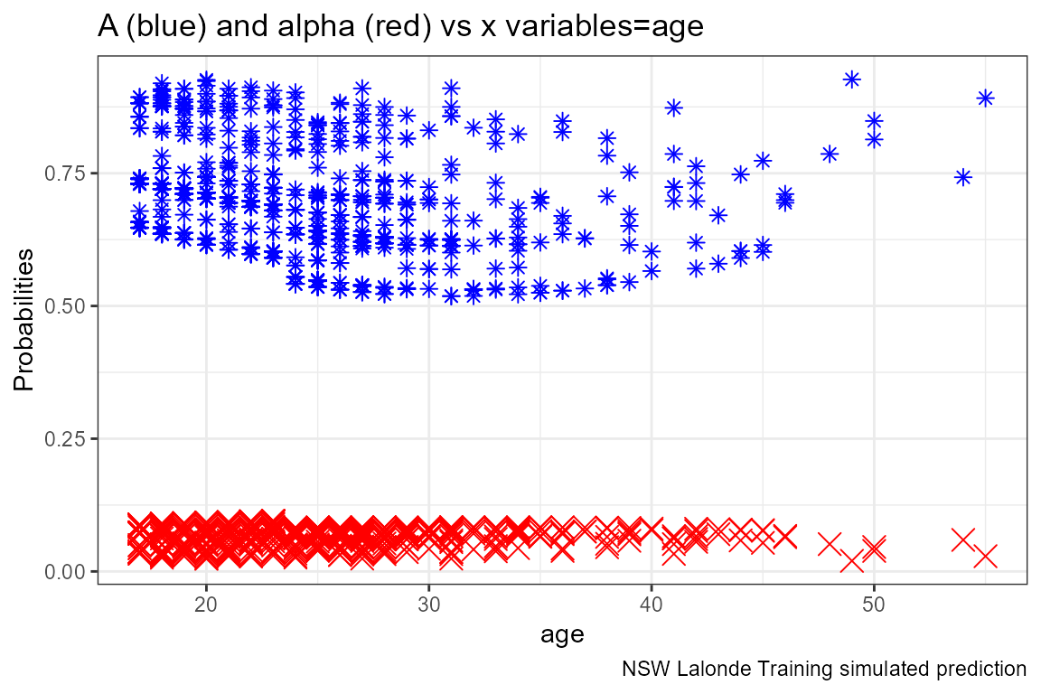
##
## [[2]]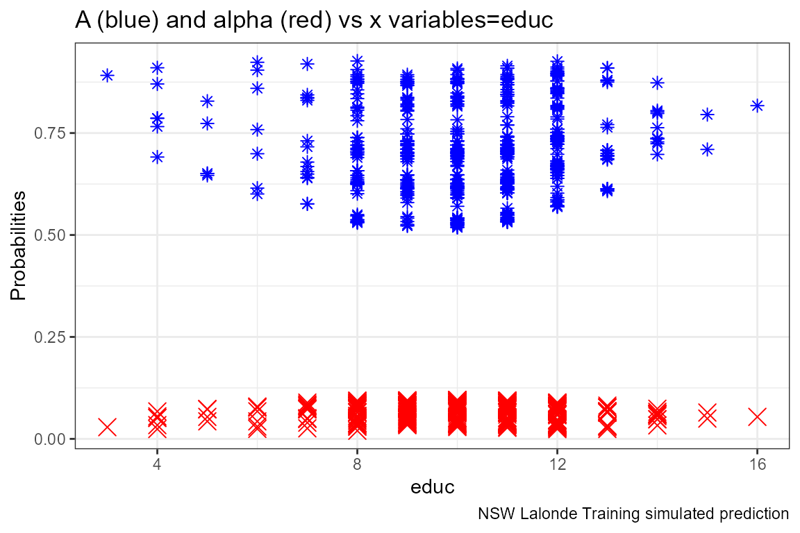
##
## [[3]]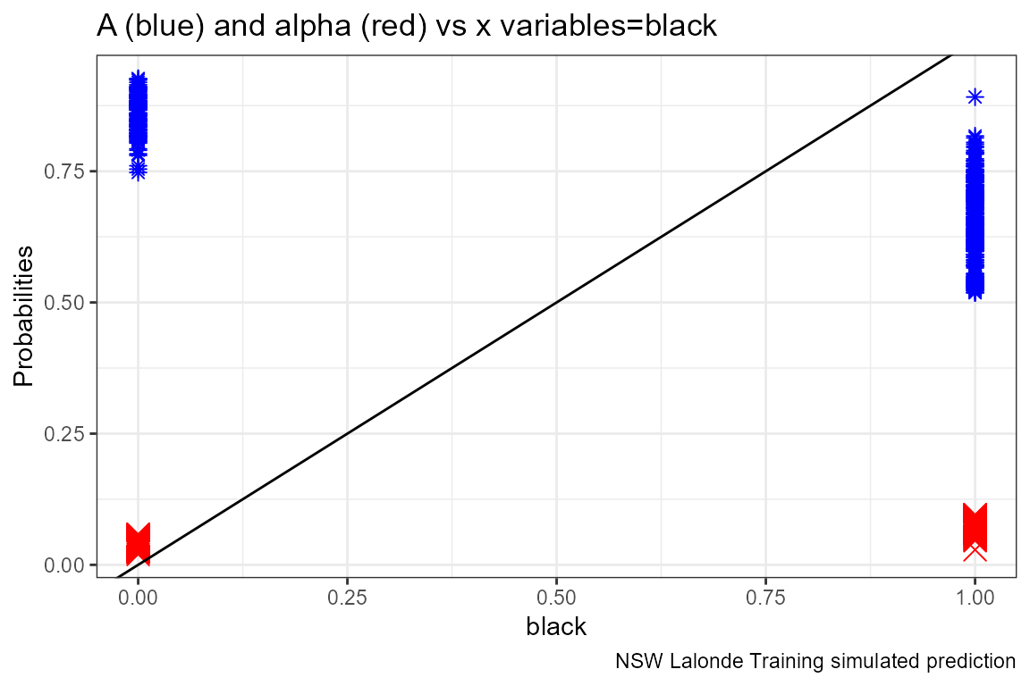
##
## [[4]]
##
## [[5]]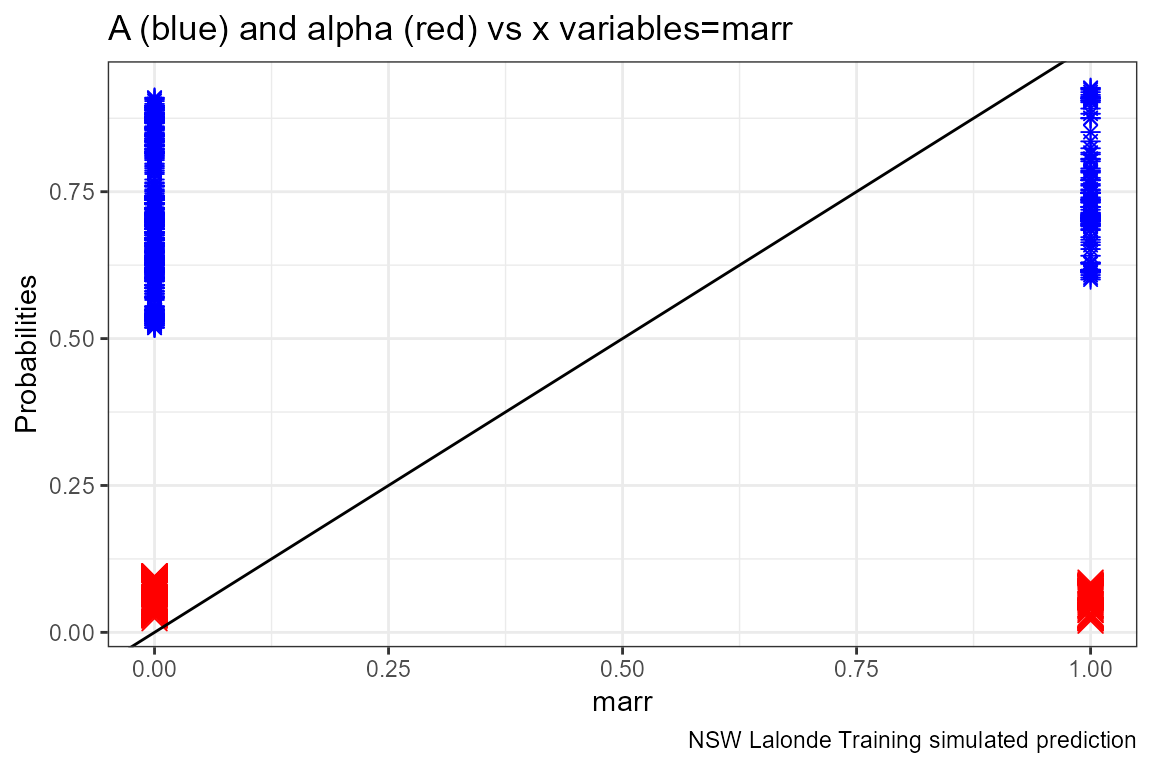
##
## [[6]]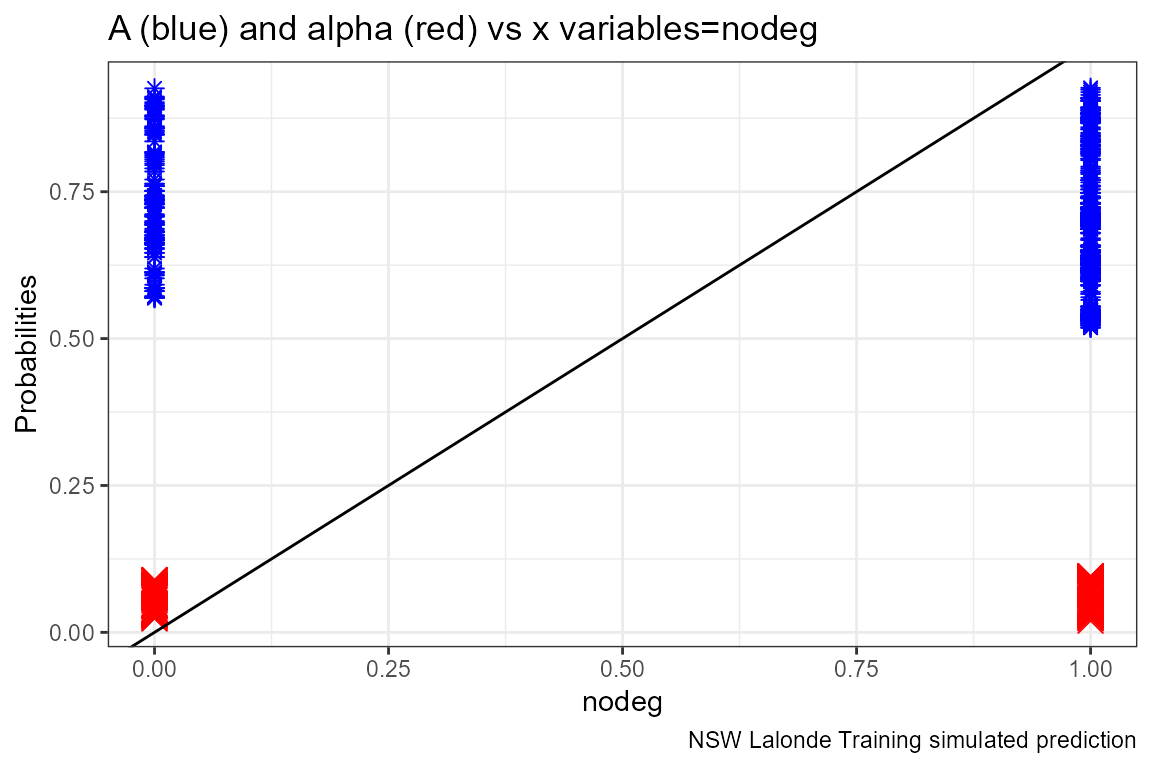
Optimal Binary Allocation
Solve for Optimal Allocations Across Preference Parameters
Invoke the binary optimal allocation function ffp_opt_anlyz_rhgin_bin that loops over rhos.
svr_inpalc <- 'rank'

beta_i <- rep(1/dim(dft)[1], times=dim(dft)[1])
dft <- cbind(dft, beta_i)
ar_rho = c(-100, -0.001,  0.95)
ar_rho <- 1 - (10^(c(seq(-2,2, length.out=30))))
ar_rho <- unique(ar_rho)

svr_rho_val <- 'rho_val'
ls_bin_solu_all_rhos <-
  ffp_opt_anlyz_rhgin_bin(dft, svr_id_i = 'id',
                          svr_A_i = 'A_i', svr_alpha_i = 'alpha_i', svr_beta_i = 'beta_i',
                          ar_rho = ar_rho,
                          svr_rho = 'rho', svr_rho_val = svr_rho_val,
                          svr_inpalc = svr_inpalc,
                          svr_expout = 'opti_exp_outcome',
                          verbose = TRUE)
## 'data.frame': 722 obs. of 54 variables:
## $ id : int 1 2 3 4 5 6 7 8 9 10 ...
## $ trt : Factor w/ 2 levels "ntran","train": 1 1 1 1 1 1 1 1 1 1 ...
## $ age : int 23 26 22 34 18 45 18 27 24 34 ...
## $ educ : int 10 12 9 9 9 11 9 12 8 11 ...
## $ black : int 1 0 1 1 1 1 1 1 0 1 ...
## $ hisp : int 0 0 0 0 0 0 0 0 0 0 ...
## $ marr : int 0 0 0 0 0 0 0 0 0 1 ...
## $ nodeg : int 1 0 1 1 1 1 1 0 1 1 ...
## $ re74 : num 0 0 0 NA 0 0 0 NA 0 0 ...
## $ re75 : num 0 0 0 4368 0 ...
## $ re78 : num 0 12384 0 14051 10740 ...
## $ re75_zero : num 1 1 1 0 1 1 1 0 1 1 ...
## $ emp78 : num 0 1 0 1 1 1 1 1 1 1 ...
## $ emp75 : num 0 0 0 1 0 0 0 1 0 0 ...
## $ race : num 1 0 1 1 1 1 1 1 0 1 ...
## $ age_m2 : num 1 2 1 2 1 2 1 2 2 2 ...
## $ age_m3 : num 2 2 2 3 1 3 1 3 2 3 ...
## $ p_mpg : num 0.678 0.89 0.688 0.638 0.704 ...
## $ p_mpg_hp : num 0.591 0.811 0.598 0.616 0.636 ...
## $ p_mpg_hp_bi0: num 0.591 0.811 0.598 0.616 0.636 ...
## $ p_mpg_hp_bi1: num 0.686 0.858 0.692 0.693 0.725 ...
## $ alpha_i : num 0.0951 0.0466 0.0943 0.0764 0.0895 ...
## $ A_i : num 0.591 0.811 0.598 0.616 0.636 ...
## $ beta_i : num 0.00139 0.00139 0.00139 0.00139 0.00139 ...
## $ rho_c1_rk : int 1 605 6 294 36 286 36 463 591 295 ...
## $ rho_c2_rk : int 1 605 6 294 36 286 36 463 591 295 ...
## $ rho_c3_rk : int 1 605 6 294 36 274 36 463 591 295 ...
## $ rho_c4_rk : int 1 605 6 294 36 274 36 463 591 295 ...
## $ rho_c5_rk : int 1 605 6 282 36 274 36 463 591 283 ...
## $ rho_c6_rk : int 1 605 6 282 36 273 36 454 591 283 ...
## $ rho_c7_rk : int 1 605 6 273 36 260 36 454 591 274 ...
## $ rho_c8_rk : int 1 605 6 268 36 260 36 454 591 269 ...
## $ rho_c9_rk : int 1 605 6 268 36 260 36 450 591 269 ...
## $ rho_c10_rk : int 1 604 6 268 36 256 36 447 591 269 ...
## $ rho_c11_rk : int 1 604 6 253 36 241 36 447 590 254 ...
## $ rho_c12_rk : int 1 604 6 246 36 230 36 444 589 247 ...
## $ rho_c13_rk : int 1 604 6 233 53 225 53 435 587 234 ...
## $ rho_c14_rk : int 1 604 6 217 90 209 90 416 587 218 ...
## $ rho_c15_rk : int 1 604 6 212 103 204 103 397 587 213 ...
## $ rho_c16_rk : int 12 604 33 211 113 203 113 375 586 212 ...
## $ rho_c17_rk : int 45 601 67 207 122 198 122 349 584 208 ...
## $ rho_c18_rk : int 64 597 73 199 124 191 124 330 584 200 ...
## $ rho_c19_rk : int 68 597 79 177 133 169 133 314 582 178 ...
## $ rho_c20_rk : int 75 593 83 155 157 147 157 307 581 156 ...
## $ rho_c21_rk : int 78 593 86 155 172 147 172 297 581 156 ...
## $ rho_c22_rk : int 81 591 92 147 181 139 181 293 579 148 ...
## $ rho_c23_rk : int 87 590 94 147 197 139 197 293 579 148 ...
## $ rho_c24_rk : int 87 589 94 147 198 138 198 292 578 148 ...
## $ rho_c25_rk : int 87 588 94 146 202 138 202 292 578 147 ...
## $ rho_c26_rk : int 87 588 94 146 206 136 206 292 578 147 ...
## $ rho_c27_rk : int 88 588 94 146 210 133 210 290 578 147 ...
## $ rho_c28_rk : int 88 588 94 146 210 133 210 290 578 147 ...
## $ rho_c29_rk : int 88 588 94 146 210 133 210 290 578 147 ...
## $ rho_c30_rk : int 88 587 94 146 210 133 210 290 578 147 ...## Joining, by = "id"
df_all_rho <- ls_bin_solu_all_rhos$df_all_rho
df_all_rho_long <- ls_bin_solu_all_rhos$df_all_rho_long

# How many people have different ranks across rhos
it_how_many_vary_rank <- sum(df_all_rho$rank_max - df_all_rho$rank_min)
it_how_many_vary_rank
## [1] -76274Change in Rank along rho
# get rank when wage rho = 1
df_all_rho_rho_c1 <- df_all_rho %>% select(id, rho_c1_rk)
# Merge
df_all_rho_long_more <- df_all_rho_long %>% mutate(rho = as.numeric(rho)) %>%
                      left_join(df_all_rho_rho_c1, by='id')
# Select subset to graph
df_rank_graph <- df_all_rho_long_more %>%
                    mutate(id = factor(id)) %>%
                    filter((id == 1) |  # utilitarian rank = 1
                           (id == 711) |  # utilitarian rank = 101
                           (id == 731)  |  # utilitarian rank = 207
                           (id == 50) |  # utilitarian rank = 300
                           (id == 1571)|  # utilitarian rank = 402
                           (id == 22) |  # utilitarian rank = 500
                           (id == 164) |  # utilitarian rank = 600
                           (id == 296)   # utilitarian rank = 701
                             ) %>%
                    mutate(one_minus_rho = 1 - !!sym(svr_rho_val)) %>%
                    mutate(rho_c1_rk = factor(rho_c1_rk))

df_rank_graph$rho_c1_rk
## [1] 1 1 1 1 1 1 1 1 1 1 1 1 1 1 1 1 1 1
## [19] 1 1 1 1 1 1 1 1 1 1 1 1 500 500 500 500 500 500
## [37] 500 500 500 500 500 500 500 500 500 500 500 500 500 500 500 500 500 500
## [55] 500 500 500 500 500 500 300 300 300 300 300 300 300 300 300 300 300 300
## [73] 300 300 300 300 300 300 300 300 300 300 300 300 300 300 300 300 300 300
## [91] 600 600 600 600 600 600 600 600 600 600 600 600 600 600 600 600 600 600
## [109] 600 600 600 600 600 600 600 600 600 600 600 600 700 700 700 700 700 700
## [127] 700 700 700 700 700 700 700 700 700 700 700 700 700 700 700 700 700 700
## [145] 700 700 700 700 700 700 101 101 101 101 101 101 101 101 101 101 101 101
## [163] 101 101 101 101 101 101 101 101 101 101 101 101 101 101 101 101 101 101
## [181] 207 207 207 207 207 207 207 207 207 207 207 207 207 207 207 207 207 207
## [199] 207 207 207 207 207 207 207 207 207 207 207 207 402 402 402 402 402 402
## [217] 402 402 402 402 402 402 402 402 402 402 402 402 402 402 402 402 402 402
## [235] 402 402 402 402 402 402
## Levels: 1 101 207 300 402 500 600 700
df_rank_graph$id <- factor(df_rank_graph$rho_c1_rk,
                           labels = c('Rank= 1  ', #200
                                      'Rank= 101', #110
                                      'Rank= 201', #95
                                      'Rank= 301', #217
                                      'Rank= 401', #274
                                      'Rank= 501', #101
                                      'Rank= 601', #131
                                      'Rank= 701' #3610
                                       ))

# x-labels
x.labels <- c('λ=0.99', 'λ=0.90', 'λ=0', 'λ=-10', 'λ=-100')
x.breaks <- c(0.01, 0.10, 1, 10, 100)

# title line 2
st_title <- sprintf("Positions on the Optimal (Binary) Allocation Queue at Varying λ Levels")
title_line2 <- sprintf("Colored lines = different individuals from the NSW training dataset")
title_line3 <- sprintf("Track ranking changes for eight individuals ranked 1, 101, ..., 701 at λ=0.99")

# Graph Results--Draw
line.plot <- df_rank_graph %>%
  ggplot(aes(x=one_minus_rho, y=!!sym(svr_inpalc),
             group=fct_rev(id),
             colour=fct_rev(id), size=2)) +
  # geom_line(aes(linetype =fct_rev(id)), size=0.75) +
  geom_line(size=0.5) +
  geom_vline(xintercept=c(1), linetype="dotted") +
  labs(title = st_title, subtitle = paste0(title_line2, '\n', title_line3),
       x = 'log10 Rescale of λ, Log10(1-λ)\nλ=1 Utilitarian (Maximize Average), λ=-infty Rawlsian (Maximize Minimum)',
       y = 'Optimal Allocation Queue Rank (1=highest)',
       caption = 'Based on a logistic regression of the employment effects of a training RCT. Data: Lalonde (AER, 1986).') +
  scale_x_continuous(trans='log10', labels = x.labels, breaks = x.breaks) +
  theme_bw(base_size=8)

# Labeling
line.plot$labels$colour <- "At λ=0.99, i's"

# Print
print(line.plot)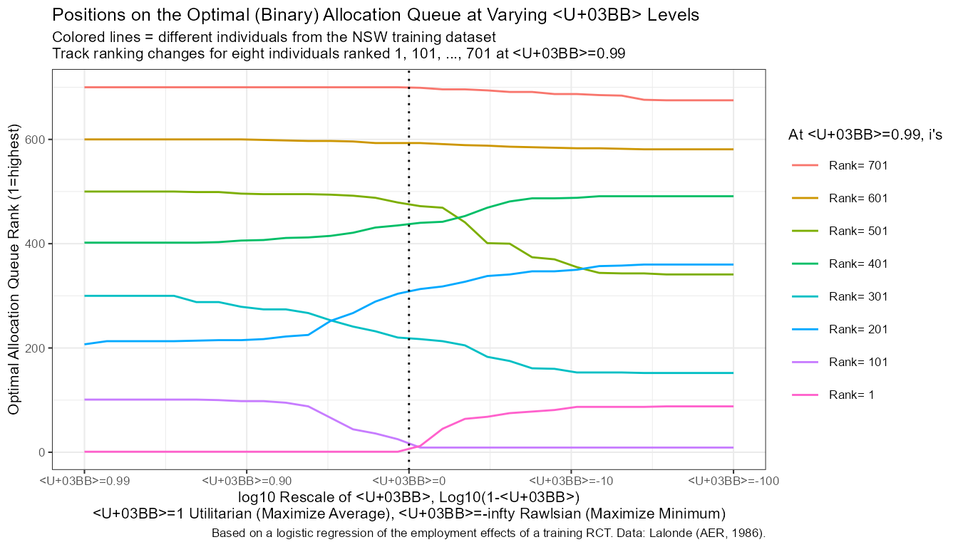
if (bl_save_img) {
  snm_cnts <- 'Lalonde_employ_rank.png'
  png(paste0(spt_img_save, snm_cnts),
        width = 135, height = 96, units='mm', res = 300, pointsize=7)
  print(line.plot)
  dev.off()
  png(paste0(spt_img_save_draft, snm_cnts),
        width = 135, height = 96, units='mm', res = 300,
      pointsize=5)
  print(line.plot)
  dev.off()
}
Save Results
# Change Variable names so that this can becombined with logit file later
df_all_rho <- df_all_rho %>% rename_at(vars(starts_with("rho_")), funs(str_replace(., "rk", "rk_employ")))
## Warning: `funs()` was deprecated in dplyr 0.8.0.
## Please use a list of either functions or lambdas:
##
## # Simple named list:
## list(mean = mean, median = median)
##
## # Auto named with `tibble::lst()`:
## tibble::lst(mean, median)
##
## # Using lambdas
## list(~ mean(., trim = .2), ~ median(., na.rm = TRUE))
## This warning is displayed once every 8 hours.
## Call `lifecycle::last_lifecycle_warnings()` to see where this warning was generated.
df_all_rho <- df_all_rho %>%
        rename(A_i_employ = A_i, alpha_i_employ = alpha_i, beta_i_employ = beta_i,
               rank_min_employ = rank_min, rank_max_employ = rank_max, avg_rank_employ = avg_rank)

# Save File
if (bl_save_rda) {
  df_opt_lalonde_training_employ <- df_all_rho
  usethis::use_data(df_opt_lalonde_training_employ, df_opt_lalonde_training_employ, overwrite = TRUE)
}
Binary Marginal Effects and Prediction without Binary
What is the relationship between ranking,
# ggplot.A.alpha.x <- function(svr_x, df,
#                              svr_alpha = 'alpha_i', svr_A = "A_i"){
#
#   scatter <- ggplot(df, aes(x=!!sym(svr_x))) +
#         geom_point(aes(y=alpha_i), size=4, shape=4, color="red") +
#         geom_point(aes(y=A_i), size=2, shape=8, color="blue") +
#         geom_abline(intercept = 0, slope = 1) + # 45 degree line
#         labs(title = paste0('A (blue) and alpha (red) vs x variables=', svr_x),
#              x = svr_x,
#              y = 'Probabilities',
#              caption = paste0(sdt_name, ' simulated prediction')) +
#         theme_bw()
#
# return(scatter)
# }