Line by Line Test Lower-Bounded Linear-Continuous Allocation with Linear Regression
Source:vignettes/ffv_opt_solin_relow_allrw.Rmd
ffv_opt_solin_relow_allrw.RmdTest lower-bounded linear-continuous optimal allocation solution line by line without function. Use the Guatemala-Cebu scrambled nutrition and height early childhood data. Regress the effect of nutritional supplements on height.
The objective of this file is to solve the linear \(N_i\) and \(H_i\) problem without invoking any functions. This function first tested out the linear solution algorithm.
File name ffv_opt_solin_relow_allrw:
- opt: optimal allocation project
- solin: linear production function
- relow: solution method relying on relative allocation against lowest (first) to receive subsidy
- allrw: all code line by line raw original file
Input and Output
There is a dataset with child attributes, nutritional inputs and outputs. Run regression to estimate some input output relationship first. Then generate required inputs for code.
- Required Input
- @param df tibble data table including variables using svr names below each row is potentially an individual who will receive alternative allocations
- @param svr_A_i string name of the A_i variable, dot product of covariates and coefficients
- @param svr_alpha_i string name of the alpha_i variable, individual specific elasticity information
- @param svr_beta_i string name of the beta_i variable, relative preference weight for each child
- @param svr_N_i string name of the vector of existing inputs, based on which to compute aggregate resource
- @param fl_N_hat float total resource avaible for allocation, if not specific, sum by svr_N_i
- @param fl_rho float preference for equality for the planner
- @return a dataframe that expands the df inputs with additional results.
- The structure assumes some regression has already taken place to generate the i specific variables listed. and
Doing this allows for lagged intereaction that are time specific in an arbitrary way.
Load Packages and Data
Load Data
Generate four categories by initial height and mother’s education levels combinations.
# Load Library

# Select Cebu Only
df_hw_cebu_m24 <- df_hgt_wgt %>% filter(S.country == 'Cebu' & svymthRound == 24 & prot > 0 & hgt > 0) %>% drop_na()

# Generate Discrete Version of momEdu
df_hw_cebu_m24 <- df_hw_cebu_m24 %>%
    mutate(momEduRound = cut(momEdu,
                             breaks=c(-Inf, 10, Inf),
                             labels=c("MEduLow","MEduHigh"))) %>%
    mutate(hgt0med = cut(hgt0,
                             breaks=c(-Inf, 50, Inf),
                             labels=c("h0low","h0high")))

df_hw_cebu_m24$momEduRound = as.factor(df_hw_cebu_m24$momEduRound)
df_hw_cebu_m24$hgt0med = as.factor(df_hw_cebu_m24$hgt0med)

# Attach
attach(df_hw_cebu_m24)
Regression with Data and Construct Input Arrays
Linear Regression
Estimation Production functions or any other function. Below, Regression height outcomes on input interacted with the categories created before. This will generate category specific marginal effects.
# Input Matrix
mt_lincv <- model.matrix(~ hgt0 + wgt0)
mt_linht <- model.matrix(~ sex:hgt0med - 1)

# Regress Height At Month 24 on Nutritional Inputs with controls
rs_hgt_prot_lin = lm(hgt ~ prot:mt_linht + mt_lincv - 1)
print(summary(rs_hgt_prot_lin))
##
## Call:
## lm(formula = hgt ~ prot:mt_linht + mt_lincv - 1)
##
## Residuals:
## Min 1Q Median 3Q Max
## -15.212 -2.339 0.088 2.437 9.805
##
## Coefficients:
## Estimate Std. Error t value Pr(>|t|)
## mt_lincv(Intercept) 5.638e+01 3.683e+00 15.307 < 2e-16 ***
## mt_lincvhgt0 3.774e-01 8.723e-02 4.326 1.66e-05 ***
## mt_lincvwgt0 1.154e-03 3.705e-04 3.115 0.00189 **
## prot:mt_linhtsexFemale:hgt0medh0low 1.014e-02 1.058e-02 0.959 0.33783
## prot:mt_linhtsexMale:hgt0medh0low 6.018e-02 9.625e-03 6.252 5.91e-10 ***
## prot:mt_linhtsexFemale:hgt0medh0high 3.228e-02 1.332e-02 2.423 0.01558 *
## prot:mt_linhtsexMale:hgt0medh0high 6.619e-02 1.001e-02 6.612 6.05e-11 ***
## ---
## Signif. codes: 0 '***' 0.001 '**' 0.01 '*' 0.05 '.' 0.1 ' ' 1
##
## Residual standard error: 3.473 on 1036 degrees of freedom
## Multiple R-squared: 0.9981, Adjusted R-squared: 0.9981
## F-statistic: 7.79e+04 on 7 and 1036 DF, p-value: < 2.2e-16
rs_hgt_prot_lin_tidy = tidy(rs_hgt_prot_lin)Log-Linear Regression
Now log-linear regressions, where inptut coefficient differs by input groups.
# Input Matrix Generation
mt_logcv <- model.matrix(~ hgt0 + wgt0)
mt_loght <- model.matrix(~ sex:hgt0med - 1)

# Log and log regression for month 24
rs_hgt_prot_log = lm(log(hgt) ~ log(prot):mt_loght + mt_logcv - 1)
print(summary(rs_hgt_prot_log))
##
## Call:
## lm(formula = log(hgt) ~ log(prot):mt_loght + mt_logcv - 1)
##
## Residuals:
## Min 1Q Median 3Q Max
## -0.223890 -0.030027 0.002461 0.031047 0.118097
##
## Coefficients:
## Estimate Std. Error t value Pr(>|t|)
## mt_logcv(Intercept) 4.087e+00 5.342e-02 76.512 < 2e-16
## mt_logcvhgt0 4.305e-03 1.224e-03 3.516 0.000457
## mt_logcvwgt0 1.465e-05 4.733e-06 3.096 0.002012
## log(prot):mt_loghtsexFemale:hgt0medh0low 6.687e-03 2.218e-03 3.014 0.002640
## log(prot):mt_loghtsexMale:hgt0medh0low 1.209e-02 2.176e-03 5.557 3.49e-08
## log(prot):mt_loghtsexFemale:hgt0medh0high 9.251e-03 2.441e-03 3.790 0.000159
## log(prot):mt_loghtsexMale:hgt0medh0high 1.394e-02 2.288e-03 6.094 1.55e-09
##
## mt_logcv(Intercept) ***
## mt_logcvhgt0 ***
## mt_logcvwgt0 **
## log(prot):mt_loghtsexFemale:hgt0medh0low **
## log(prot):mt_loghtsexMale:hgt0medh0low ***
## log(prot):mt_loghtsexFemale:hgt0medh0high ***
## log(prot):mt_loghtsexMale:hgt0medh0high ***
## ---
## Signif. codes: 0 '***' 0.001 '**' 0.01 '*' 0.05 '.' 0.1 ' ' 1
##
## Residual standard error: 0.04436 on 1036 degrees of freedom
## Multiple R-squared: 0.9999, Adjusted R-squared: 0.9999
## F-statistic: 1.448e+06 on 7 and 1036 DF, p-value: < 2.2e-16
rs_hgt_prot_log_tidy = tidy(rs_hgt_prot_log)Construct Input Arrays \(A_i\) and \(\alpha_i\)
Multiply coefficient vector by covariate matrix to generate A vector that is child/individual specific.
# Generate A_i
ar_Ai_lin <- mt_lincv %*% as.matrix(rs_hgt_prot_lin_tidy %>% filter(!str_detect(term, 'prot')) %>% select(estimate))
ar_Ai_log <- mt_logcv %*% as.matrix(rs_hgt_prot_log_tidy %>% filter(!str_detect(term, 'prot')) %>% select(estimate))

# Generate alpha_i
ar_alphai_lin <- mt_linht %*% as.matrix(rs_hgt_prot_lin_tidy %>% filter(str_detect(term, 'prot')) %>% select(estimate))
ar_alphai_log <- mt_loght %*% as.matrix(rs_hgt_prot_log_tidy %>% filter(str_detect(term, 'prot')) %>% select(estimate))

# Child Weight
ar_beta <- rep(1/length(ar_Ai_lin), times=length(ar_Ai_lin))

# Initate Dataframe that will store all estimates and optimal allocation relevant information
# combine identifying key information along with estimation A, alpha results
# note that we only need indi.id as key
mt_opti <- cbind(ar_alphai_lin, ar_Ai_lin, ar_beta)
ar_st_varnames <- c('alpha', 'A', 'beta')
df_esti_alpha_A_beta <- as_tibble(mt_opti) %>% rename_all(~c(ar_st_varnames))
## Warning: The `x` argument of `as_tibble.matrix()` must have unique column names if `.name_repair` is omitted as of tibble 2.0.0.
## Using compatibility `.name_repair`.
## This warning is displayed once every 8 hours.
## Call `lifecycle::last_lifecycle_warnings()` to see where this warning was generated.
tb_key_alpha_A_beta <- bind_cols(df_hw_cebu_m24, df_esti_alpha_A_beta) %>%
              select(one_of(c('S.country', 'vil.id', 'indi.id', 'svymthRound', ar_st_varnames)))

# Unique beta, A, and alpha groups
tb_opti_unique <- tb_key_alpha_A_beta %>% group_by(!!!syms(ar_st_varnames)) %>%
                    arrange(!!!syms(ar_st_varnames)) %>%
                    summarise(n_obs_group=n())
## `summarise()` has grouped output by 'alpha', 'A'. You can override using the `.groups` argument.Optimal Linear Allocations
Parameters for Optimal Allocation
# Child Count
df_hw_cebu_m24_full <- df_hw_cebu_m24
it_obs = dim(df_hw_cebu_m24)[1]

# Total Resource Count
ar_prot_data = df_hw_cebu_m24$prot
fl_N_agg = sum(ar_prot_data)

# Vector of Planner Preference
ar_rho <- c(-100, 0.8)
ar_rho <- c(-50, -25, -10)
ar_rho <- c(-100, -5, -1, 0.1, 0.6, 0.8)
ar_rho <- c(seq(-200, -100, length.out=5), seq(-100, -25, length.out=5), seq(-25, -5, length.out=5), seq(-5, -1, length.out=5), seq(-1, -0.01, length.out=5), seq(0.01, 0.25, length.out=5), seq(0.25, 0.90, length.out=5))
ar_rho <- unique(ar_rho)
Optimal Linear Allocation (CRS)
This also works with any CRS CES.
# Optimal Linear Equation

# accumulate allocation results
tb_opti_alloc_all_rho <- tb_key_alpha_A_beta

# A. First Loop over Planner Preference
# Generate Rank Order
for (it_rho_ctr in seq(1,length(ar_rho))) {
  rho = ar_rho[it_rho_ctr]

  # B. Generate V4, Rank Index Value, rho specific
  # tb_opti <- tb_opti %>% mutate(!!paste0('rv_', it_rho_ctr) := A/((alpha*beta))^(1/(1-rho)))
  tb_opti <- tb_key_alpha_A_beta %>% mutate(rank_val = A/((alpha*beta))^(1/(1-rho)))

  # c. Generate Rank Index
  tb_opti <- tb_opti %>% arrange(rank_val) %>% mutate(rank_idx = row_number())

  # d. Populate lowest index alpha, beta, and A to all rows
  tb_opti <- tb_opti %>% mutate(lowest_rank_A = A[rank_idx==1]) %>%
                mutate(lowest_rank_alpha = alpha[rank_idx==1]) %>%
                mutate(lowest_rank_beta = beta[rank_idx==1])

  # e. relative slope and relative intercept with respect to lowest index
  tb_opti <- tb_opti %>%
                mutate(rela_slope_to_lowest =
                         (((lowest_rank_alpha*lowest_rank_beta)/(alpha*beta))^(1/(rho-1))*(lowest_rank_alpha/alpha))
                      ) %>%
                mutate(rela_intercept_to_lowest =
                         ((((lowest_rank_alpha*lowest_rank_beta)/(alpha*beta))^(1/(rho-1))*(lowest_rank_A/alpha)) - (A/alpha))
                      )

  # f. cumulative sums
  tb_opti <- tb_opti %>%
                mutate(rela_slope_to_lowest_cumsum =
                         cumsum(rela_slope_to_lowest)
                      ) %>%
                mutate(rela_intercept_to_lowest_cumsum =
                         cumsum(rela_intercept_to_lowest)
                      )

  # g. inverting cumulative slopes and intercepts
  tb_opti <- tb_opti %>%
                mutate(rela_slope_to_lowest_cumsum_invert =
                         (1/rela_slope_to_lowest_cumsum)
                      ) %>%
                mutate(rela_intercept_to_lowest_cumsum_invert =
                         ((-1)*(rela_intercept_to_lowest_cumsum)/(rela_slope_to_lowest_cumsum))
                      )

  # h. Relative x-intercept points
  tb_opti <- tb_opti %>%
                mutate(rela_x_intercept =
                         (-1)*(rela_intercept_to_lowest/rela_slope_to_lowest)
                      )

  # i. Inverted relative x-intercepts
  tb_opti <- tb_opti %>%
                mutate(opti_lowest_spline_knots =
                         (rela_intercept_to_lowest_cumsum + rela_slope_to_lowest_cumsum*rela_x_intercept)
                      )

  # j. Sort by order of receiving transfers/subsidies
  tb_opti <- tb_opti %>% arrange(rela_x_intercept)

  # k. Find position of subsidy
  tb_opti <- tb_opti %>% arrange(opti_lowest_spline_knots) %>%
                mutate(tot_devi = opti_lowest_spline_knots - fl_N_agg) %>%
                arrange((-1)*case_when(tot_devi < 0 ~ tot_devi)) %>%
                mutate(allocate_lowest =
                         case_when(row_number() == 1 ~
                                     rela_intercept_to_lowest_cumsum_invert +
                                     rela_slope_to_lowest_cumsum_invert*fl_N_agg)) %>%
                mutate(allocate_lowest = allocate_lowest[row_number() == 1]) %>%
                mutate(opti_allocate =
                         rela_intercept_to_lowest +
                         rela_slope_to_lowest*allocate_lowest) %>%
                mutate(opti_allocate =
                         case_when(opti_allocate >= 0 ~ opti_allocate, TRUE ~ 0)) %>%
                mutate(allocate_total = sum(opti_allocate, na.rm=TRUE))

  # l. Predictes Expected choice: A + alpha*opti_allocate
  tb_opti <- tb_opti %>% mutate(opti_exp_outcome = A + alpha*opti_allocate)

  # m. Keep for df collection individual key + optimal allocation
  # _on stands for optimal nutritional choices
  # _eh stands for expected height
  tb_opti_main_results <- tb_opti %>%
    select(-one_of(c('lowest_rank_alpha', 'lowest_rank_beta')))
  tb_opti_allocate_wth_key <- tb_opti %>% select(one_of('indi.id','opti_allocate', 'opti_exp_outcome')) %>%
                                rename(!!paste0('rho_c', it_rho_ctr, '_on') := !!sym('opti_allocate'),
                                       !!paste0('rho_c', it_rho_ctr, '_eh') := !!sym('opti_exp_outcome'))

  # n. merge optimal allocaiton results from different planner preference
  tb_opti_alloc_all_rho <- tb_opti_alloc_all_rho %>% left_join(tb_opti_allocate_wth_key, by='indi.id')

  # print subset
  if (it_rho_ctr == 1 | it_rho_ctr == length(ar_rho) | it_rho_ctr == round(length(ar_rho)/2)) {
    print('')
    print('xxxxxxxxxxxxxxxxxxxxxxxxxxxxxxxxxxxxxxxxxxxxxxxxx')
    print(paste0('xxx rho:', rho))
    print('xxxxxxxxxxxxxxxxxxxxxxxxxxxxxxxxxxxxxxxxxxxxxxxxx')
    print('xxxxxxxxxxxxxxxxxxxxxxxxxxxxxxxxxxxxxxxxxxxxxxxxx')

    print(summary(tb_opti_main_results))
  }
}
## [1] ""
## [1] "xxxxxxxxxxxxxxxxxxxxxxxxxxxxxxxxxxxxxxxxxxxxxxxxx"
## [1] "xxx rho:-200"
## [1] "xxxxxxxxxxxxxxxxxxxxxxxxxxxxxxxxxxxxxxxxxxxxxxxxx"
## [1] "xxxxxxxxxxxxxxxxxxxxxxxxxxxxxxxxxxxxxxxxxxxxxxxxx"
## S.country vil.id indi.id svymthRound
## Length:1043 Min. : 1.00 Min. : 2.0 Min. :24
## Class :character 1st Qu.: 7.00 1st Qu.: 298.5 1st Qu.:24
## Mode :character Median :12.00 Median : 627.0 Median :24
## Mean :12.52 Mean : 634.8 Mean :24
## 3rd Qu.:17.00 3rd Qu.: 939.5 3rd Qu.:24
## Max. :33.00 Max. :1349.0 Max. :24
## alpha A beta rank_val
## Min. :0.01014 Min. :73.70 Min. :0.0009588 Min. :77.36
## 1st Qu.:0.01014 1st Qu.:77.73 1st Qu.:0.0009588 1st Qu.:81.92
## Median :0.06018 Median :78.45 Median :0.0009588 Median :82.69
## Mean :0.04108 Mean :78.46 Mean :0.0009588 Mean :82.63
## 3rd Qu.:0.06018 3rd Qu.:79.15 3rd Qu.:0.0009588 3rd Qu.:83.34
## Max. :0.06619 Max. :84.61 Max. :0.0009588 Max. :89.09
## rank_idx lowest_rank_A rela_slope_to_lowest rela_intercept_to_lowest
## Min. : 1.0 Min. :73.7 Min. :0.9096 Min. :-638.33
## 1st Qu.: 261.5 1st Qu.:73.7 1st Qu.:1.0000 1st Qu.:-416.71
## Median : 522.0 Median :73.7 Median :1.0000 Median :-103.23
## Mean : 522.0 Mean :73.7 Mean :2.7200 Mean :-221.98
## 3rd Qu.: 782.5 3rd Qu.:73.7 3rd Qu.:5.8796 3rd Qu.: -77.34
## Max. :1043.0 Max. :73.7 Max. :5.8796 Max. : 0.00
## rela_slope_to_lowest_cumsum rela_intercept_to_lowest_cumsum
## Min. : 1.0 Min. :-231525
## 1st Qu.: 729.9 1st Qu.:-178488
## Median :1502.8 Median :-105313
## Mean :1499.0 Mean :-110538
## 3rd Qu.:2325.3 3rd Qu.: -44408
## Max. :2837.0 Max. : 0
## rela_slope_to_lowest_cumsum_invert rela_intercept_to_lowest_cumsum_invert
## Min. :0.0003525 Min. : 0.00
## 1st Qu.:0.0004300 1st Qu.:60.84
## Median :0.0006654 Median :70.08
## Mean :0.0040250 Mean :67.06
## 3rd Qu.:0.0013700 3rd Qu.:76.76
## Max. :1.0000000 Max. :81.61
## rela_x_intercept opti_lowest_spline_knots tot_devi allocate_lowest
## Min. : 0.00 Min. : 0 Min. :-22823 Min. :85.24
## 1st Qu.: 72.17 1st Qu.: 8275 1st Qu.:-14548 1st Qu.:85.24
## Median : 84.37 Median : 21478 Median : -1345 Median :85.24
## Mean : 83.42 Mean : 29824 Mean : 7002 Mean :85.24
## 3rd Qu.: 94.53 3rd Qu.: 41314 3rd Qu.: 18491 3rd Qu.:85.24
## Max. :185.68 Max. :295234 Max. :272412 Max. :85.24
## opti_allocate allocate_total opti_exp_outcome
## Min. : 0.000 Min. :22823 Min. :78.13
## 1st Qu.: 0.000 1st Qu.:22823 1st Qu.:78.36
## Median : 1.289 Median :22823 Median :78.83
## Mean : 21.882 Mean :22823 Mean :78.94
## 3rd Qu.: 21.838 3rd Qu.:22823 3rd Qu.:79.15
## Max. :371.159 Max. :22823 Max. :84.61
## [1] ""
## [1] "xxxxxxxxxxxxxxxxxxxxxxxxxxxxxxxxxxxxxxxxxxxxxxxxx"
## [1] "xxx rho:-3"
## [1] "xxxxxxxxxxxxxxxxxxxxxxxxxxxxxxxxxxxxxxxxxxxxxxxxx"
## [1] "xxxxxxxxxxxxxxxxxxxxxxxxxxxxxxxxxxxxxxxxxxxxxxxxx"
## S.country vil.id indi.id svymthRound
## Length:1043 Min. : 1.00 Min. : 2.0 Min. :24
## Class :character 1st Qu.: 7.00 1st Qu.: 298.5 1st Qu.:24
## Mode :character Median :12.00 Median : 627.0 Median :24
## Mean :12.52 Mean : 634.8 Mean :24
## 3rd Qu.:17.00 3rd Qu.: 939.5 3rd Qu.:24
## Max. :33.00 Max. :1349.0 Max. :24
## alpha A beta rank_val
## Min. :0.01014 Min. :73.70 Min. :0.0009588 Min. : 845.6
## 1st Qu.:0.01014 1st Qu.:77.73 1st Qu.:0.0009588 1st Qu.: 892.2
## Median :0.06018 Median :78.45 Median :0.0009588 Median : 906.5
## Mean :0.04108 Mean :78.46 Mean :0.0009588 Mean :1082.8
## 3rd Qu.:0.06018 3rd Qu.:79.15 3rd Qu.:0.0009588 3rd Qu.:1383.7
## Max. :0.06619 Max. :84.61 Max. :0.0009588 Max. :1424.0
## rank_idx lowest_rank_A rela_slope_to_lowest rela_intercept_to_lowest
## Min. : 1.0 Min. :73.7 Min. :0.931 Min. :-3183.95
## 1st Qu.: 261.5 1st Qu.:73.7 1st Qu.:1.000 1st Qu.:-2962.33
## Median : 522.0 Median :73.7 Median :1.000 Median : -85.91
## Mean : 522.0 Mean :73.7 Mean :1.997 Mean :-1106.86
## 3rd Qu.: 782.5 3rd Qu.:73.7 3rd Qu.:3.801 3rd Qu.: -65.38
## Max. :1043.0 Max. :73.7 Max. :3.801 Max. : 0.00
## rela_slope_to_lowest_cumsum rela_intercept_to_lowest_cumsum
## Min. : 1.0 Min. :-1154457
## 1st Qu.: 252.2 1st Qu.: -360111
## Median : 507.3 Median : -33998
## Mean : 705.8 Mean : -226709
## 3rd Qu.:1093.2 3rd Qu.: -14454
## Max. :2083.4 Max. : 0
## rela_slope_to_lowest_cumsum_invert rela_intercept_to_lowest_cumsum_invert
## Min. :0.0004800 Min. : 0.00
## 1st Qu.:0.0009147 1st Qu.: 57.32
## Median :0.0019712 Median : 67.02
## Mean :0.0071664 Mean :180.86
## 3rd Qu.:0.0039658 3rd Qu.:329.40
## Max. :1.0000000 Max. :554.13
## rela_x_intercept opti_lowest_spline_knots tot_devi allocate_lowest
## Min. : 0.00 Min. : 0 Min. :-22823 Min. :111
## 1st Qu.: 67.55 1st Qu.: 2579 1st Qu.:-20244 1st Qu.:111
## Median : 88.18 Median : 10738 Median :-12085 Median :111
## Mean :343.58 Mean :191130 Mean :168308 Mean :111
## 3rd Qu.:779.36 3rd Qu.:491900 3rd Qu.:469077 3rd Qu.:111
## Max. :837.66 Max. :590710 Max. :567888 Max. :111
## opti_allocate allocate_total opti_exp_outcome
## Min. : 0.00 Min. :22823 Min. :74.37
## 1st Qu.: 0.00 1st Qu.:22823 1st Qu.:78.35
## Median : 21.29 Median :22823 Median :80.38
## Mean : 21.88 Mean :22823 Mean :79.83
## 3rd Qu.: 41.90 3rd Qu.:22823 3rd Qu.:80.38
## Max. :111.04 Max. :22823 Max. :84.61
## [1] ""
## [1] "xxxxxxxxxxxxxxxxxxxxxxxxxxxxxxxxxxxxxxxxxxxxxxxxx"
## [1] "xxx rho:0.9"
## [1] "xxxxxxxxxxxxxxxxxxxxxxxxxxxxxxxxxxxxxxxxxxxxxxxxx"
## [1] "xxxxxxxxxxxxxxxxxxxxxxxxxxxxxxxxxxxxxxxxxxxxxxxxx"
## S.country vil.id indi.id svymthRound
## Length:1043 Min. : 1.00 Min. : 2.0 Min. :24
## Class :character 1st Qu.: 7.00 1st Qu.: 298.5 1st Qu.:24
## Mode :character Median :12.00 Median : 627.0 Median :24
## Mean :12.52 Mean : 634.8 Mean :24
## 3rd Qu.:17.00 3rd Qu.: 939.5 3rd Qu.:24
## Max. :33.00 Max. :1349.0 Max. :24
## alpha A beta rank_val
## Min. :0.01014 Min. :73.70 Min. :0.0009588 Min. :7.380e+43
## 1st Qu.:0.01014 1st Qu.:77.73 1st Qu.:0.0009588 1st Qu.:1.876e+44
## Median :0.06018 Median :78.45 Median :0.0009588 Median :1.926e+44
## Mean :0.04108 Mean :78.46 Mean :0.0009588 Mean :3.415e+51
## 3rd Qu.:0.06018 3rd Qu.:79.15 3rd Qu.:0.0009588 3rd Qu.:1.020e+52
## Max. :0.06619 Max. :84.61 Max. :0.0009588 Max. :1.049e+52
## rank_idx lowest_rank_A rela_slope_to_lowest rela_intercept_to_lowest
## Min. : 1.0 Min. :78.22 Min. :0.0000 Min. :-7838.9
## 1st Qu.: 261.5 1st Qu.:78.22 1st Qu.:0.0000 1st Qu.:-7617.3
## Median : 522.0 Median :78.22 Median :0.4243 Median : -807.4
## Mean : 522.0 Mean :78.22 Mean :0.3547 Mean :-3133.9
## 3rd Qu.: 782.5 3rd Qu.:78.22 3rd Qu.:0.4243 3rd Qu.: -773.1
## Max. :1043.0 Max. :78.22 Max. :1.0000 Max. : 0.0
## rela_slope_to_lowest_cumsum rela_intercept_to_lowest_cumsum
## Min. : 1.0 Min. :-3268692
## 1st Qu.:245.7 1st Qu.:-1261733
## Median :356.2 Median : -232715
## Mean :292.5 Mean : -743262
## 3rd Qu.:370.0 3rd Qu.: -25972
## Max. :370.0 Max. : 0
## rela_slope_to_lowest_cumsum_invert rela_intercept_to_lowest_cumsum_invert
## Min. :0.002703 Min. : 0.0
## 1st Qu.:0.002703 1st Qu.: 105.7
## Median :0.002808 Median : 653.3
## Mean :0.008086 Mean :2027.3
## 3rd Qu.:0.004071 3rd Qu.:3410.2
## Max. :1.000000 Max. :8834.6
## rela_x_intercept opti_lowest_spline_knots tot_devi
## Min. :0.000e+00 Min. :0.000e+00 Min. :-2.282e+04
## 1st Qu.:1.822e+03 1st Qu.:4.217e+05 1st Qu.: 3.989e+05
## Median :1.903e+03 Median :4.451e+05 Median : 4.223e+05
## Mean :5.467e+10 Mean :2.023e+13 Mean : 2.023e+13
## 3rd Qu.:1.633e+11 3rd Qu.:6.041e+13 3rd Qu.: 6.041e+13
## Max. :1.680e+11 Max. :6.217e+13 Max. : 6.217e+13
## allocate_lowest opti_allocate allocate_total opti_exp_outcome
## Min. :119.1 Min. : 0.00 Min. :22823 Min. :73.70
## 1st Qu.:119.1 1st Qu.: 0.00 1st Qu.:22823 1st Qu.:77.73
## Median :119.1 Median : 0.00 Median :22823 Median :78.46
## Mean :119.1 Mean : 21.88 Mean :22823 Mean :79.91
## 3rd Qu.:119.1 3rd Qu.: 0.00 3rd Qu.:22823 3rd Qu.:79.87
## Max. :119.1 Max. :119.06 Max. :22823 Max. :86.10## S.country vil.id indi.id svymthRound
## Length:1043 Min. : 1.00 Min. : 2.0 Min. :24
## Class :character 1st Qu.: 7.00 1st Qu.: 298.5 1st Qu.:24
## Mode :character Median :12.00 Median : 627.0 Median :24
## Mean :12.52 Mean : 634.8 Mean :24
## 3rd Qu.:17.00 3rd Qu.: 939.5 3rd Qu.:24
## Max. :33.00 Max. :1349.0 Max. :24
## alpha A beta rho_c1_on
## Min. :0.01014 Min. :73.70 Min. :0.0009588 Min. : 0.000
## 1st Qu.:0.01014 1st Qu.:77.73 1st Qu.:0.0009588 1st Qu.: 0.000
## Median :0.06018 Median :78.45 Median :0.0009588 Median : 1.289
## Mean :0.04108 Mean :78.46 Mean :0.0009588 Mean : 21.882
## 3rd Qu.:0.06018 3rd Qu.:79.15 3rd Qu.:0.0009588 3rd Qu.: 21.838
## Max. :0.06619 Max. :84.61 Max. :0.0009588 Max. :371.159
## rho_c1_eh rho_c2_on rho_c2_eh rho_c3_on
## Min. :78.13 Min. : 0.000 Min. :78.11 Min. : 0.000
## 1st Qu.:78.36 1st Qu.: 0.000 1st Qu.:78.36 1st Qu.: 0.000
## Median :78.83 Median : 2.247 Median :78.91 Median : 3.604
## Mean :78.94 Mean : 21.882 Mean :78.96 Mean : 21.882
## 3rd Qu.:79.15 3rd Qu.: 22.480 3rd Qu.:79.15 3rd Qu.: 23.625
## Max. :84.61 Max. :369.036 Max. :84.61 Max. :366.005
## rho_c3_eh rho_c4_on rho_c4_eh rho_c5_on
## Min. :78.08 Min. : 0.000 Min. :78.03 Min. : 0.000
## 1st Qu.:78.36 1st Qu.: 0.000 1st Qu.:78.36 1st Qu.: 0.000
## Median :79.01 Median : 5.173 Median :79.14 Median : 7.713
## Mean :78.99 Mean : 21.882 Mean :79.04 Mean : 21.882
## 3rd Qu.:79.15 3rd Qu.: 24.753 3rd Qu.:79.20 3rd Qu.: 26.879
## Max. :84.61 Max. :361.458 Max. :84.61 Max. :354.063
## rho_c5_eh rho_c6_on rho_c6_eh rho_c7_on
## Min. :77.96 Min. : 0.00 Min. :77.86 Min. : 0.00
## 1st Qu.:78.36 1st Qu.: 0.00 1st Qu.:78.36 1st Qu.: 0.00
## Median :79.35 Median : 9.47 Median :79.57 Median : 11.60
## Mean :79.10 Mean : 21.88 Mean :79.18 Mean : 21.88
## 3rd Qu.:79.42 3rd Qu.: 27.61 3rd Qu.:79.66 3rd Qu.: 30.74
## Max. :84.61 Max. :344.53 Max. :84.61 Max. :326.54
## rho_c7_eh rho_c8_on rho_c8_eh rho_c9_on
## Min. :77.68 Min. : 0.00 Min. :77.25 Min. : 0.00
## 1st Qu.:78.36 1st Qu.: 0.00 1st Qu.:78.36 1st Qu.: 0.00
## Median :79.89 Median : 15.29 Median :80.39 Median : 13.87
## Mean :79.31 Mean : 21.88 Mean :79.53 Mean : 21.88
## 3rd Qu.:79.89 3rd Qu.: 34.90 3rd Qu.:80.39 3rd Qu.: 40.99
## Max. :84.61 Max. :284.15 Max. :84.61 Max. :121.45
## rho_c9_eh rho_c10_on rho_c10_eh rho_c11_on
## Min. :75.60 Min. : 0.00 Min. :74.41 Min. : 0.00
## 1st Qu.:78.36 1st Qu.: 0.00 1st Qu.:78.36 1st Qu.: 0.00
## Median :80.96 Median : 12.04 Median :80.99 Median : 13.15
## Mean :79.79 Mean : 21.88 Mean :79.81 Mean : 21.88
## 3rd Qu.:80.96 3rd Qu.: 41.54 3rd Qu.:80.99 3rd Qu.: 41.19
## Max. :84.61 Max. :121.25 Max. :84.61 Max. :120.56
## rho_c11_eh rho_c12_on rho_c12_eh rho_c13_on
## Min. :74.37 Min. : 0.00 Min. :74.37 Min. : 0.00
## 1st Qu.:78.35 1st Qu.: 0.00 1st Qu.:78.35 1st Qu.: 0.00
## Median :80.95 Median : 15.17 Median :80.87 Median : 20.24
## Mean :79.82 Mean : 21.88 Mean :79.82 Mean : 21.88
## 3rd Qu.:80.95 3rd Qu.: 41.46 3rd Qu.:80.87 3rd Qu.: 41.61
## Max. :84.61 Max. :119.13 Max. :84.61 Max. :115.30
## rho_c13_eh rho_c14_on rho_c14_eh rho_c15_on
## Min. :74.37 Min. : 0.00 Min. :74.37 Min. : 0.00
## 1st Qu.:78.35 1st Qu.: 0.00 1st Qu.:78.35 1st Qu.: 0.00
## Median :80.64 Median : 22.12 Median :80.53 Median : 21.29
## Mean :79.83 Mean : 21.88 Mean :79.83 Mean : 21.88
## 3rd Qu.:80.64 3rd Qu.: 41.54 3rd Qu.:80.53 3rd Qu.: 41.90
## Max. :84.61 Max. :113.60 Max. :84.61 Max. :111.04
## rho_c15_eh rho_c16_on rho_c16_eh rho_c17_on
## Min. :74.37 Min. : 0.00 Min. :74.37 Min. : 0.00
## 1st Qu.:78.35 1st Qu.: 0.00 1st Qu.:78.35 1st Qu.: 0.00
## Median :80.38 Median : 21.41 Median :80.12 Median :13.93
## Mean :79.83 Mean : 21.88 Mean :79.84 Mean :21.88
## 3rd Qu.:80.38 3rd Qu.: 42.07 3rd Qu.:80.12 3rd Qu.:41.17
## Max. :84.61 Max. :106.76 Max. :84.61 Max. :98.14
## rho_c17_eh rho_c18_on rho_c18_eh rho_c19_on
## Min. :74.37 Min. : 0.00 Min. :74.37 Min. : 0.000
## 1st Qu.:78.35 1st Qu.: 0.00 1st Qu.:78.35 1st Qu.: 0.000
## Median :79.60 Median :10.43 Median :79.38 Median : 5.523
## Mean :79.86 Mean :21.88 Mean :79.86 Mean :21.882
## 3rd Qu.:79.87 3rd Qu.:40.28 3rd Qu.:79.87 3rd Qu.:37.688
## Max. :84.61 Max. :94.48 Max. :84.61 Max. :91.211
## rho_c19_eh rho_c20_on rho_c20_eh rho_c21_on
## Min. :74.37 Min. : 0.00 Min. :74.37 Min. : 0.00
## 1st Qu.:78.35 1st Qu.: 0.00 1st Qu.:78.35 1st Qu.: 0.00
## Median :79.09 Median : 0.00 Median :78.66 Median : 0.00
## Mean :79.87 Mean : 21.88 Mean :79.89 Mean : 21.88
## 3rd Qu.:79.87 3rd Qu.: 32.66 3rd Qu.:79.87 3rd Qu.: 19.98
## Max. :84.61 Max. :100.22 Max. :84.85 Max. :111.57
## rho_c21_eh rho_c22_on rho_c22_eh rho_c23_on
## Min. :74.37 Min. : 0.00 Min. :74.37 Min. : 0.00
## 1st Qu.:77.90 1st Qu.: 0.00 1st Qu.:77.81 1st Qu.: 0.00
## Median :78.46 Median : 0.00 Median :78.46 Median : 0.00
## Mean :79.90 Mean : 21.88 Mean :79.90 Mean : 21.88
## 3rd Qu.:79.87 3rd Qu.: 18.42 3rd Qu.:79.87 3rd Qu.: 12.89
## Max. :85.60 Max. :112.48 Max. :85.66 Max. :114.96
## rho_c23_eh rho_c24_on rho_c24_eh rho_c25_on
## Min. :74.37 Min. : 0.000 Min. :74.37 Min. : 0.00
## 1st Qu.:77.73 1st Qu.: 0.000 1st Qu.:77.73 1st Qu.: 0.00
## Median :78.46 Median : 0.000 Median :78.46 Median : 0.00
## Mean :79.91 Mean : 21.882 Mean :79.91 Mean : 21.88
## 3rd Qu.:79.87 3rd Qu.: 5.622 3rd Qu.:79.87 3rd Qu.: 0.00
## Max. :85.83 Max. :116.787 Max. :85.95 Max. :118.02
## rho_c25_eh rho_c26_on rho_c26_eh rho_c27_on
## Min. :74.37 Min. : 0.00 Min. :74.37 Min. : 0.00
## 1st Qu.:77.73 1st Qu.: 0.00 1st Qu.:77.73 1st Qu.: 0.00
## Median :78.46 Median : 0.00 Median :78.46 Median : 0.00
## Mean :79.91 Mean : 21.88 Mean :79.91 Mean : 21.88
## 3rd Qu.:79.87 3rd Qu.: 0.00 3rd Qu.:79.87 3rd Qu.: 0.00
## Max. :86.03 Max. :118.63 Max. :86.07 Max. :119.06
## rho_c27_eh rho_c28_on rho_c28_eh rho_c29_on
## Min. :73.70 Min. : 0.00 Min. :73.70 Min. : 0.00
## 1st Qu.:77.73 1st Qu.: 0.00 1st Qu.:77.73 1st Qu.: 0.00
## Median :78.46 Median : 0.00 Median :78.46 Median : 0.00
## Mean :79.91 Mean : 21.88 Mean :79.91 Mean : 21.88
## 3rd Qu.:79.87 3rd Qu.: 0.00 3rd Qu.:79.87 3rd Qu.: 0.00
## Max. :86.10 Max. :119.06 Max. :86.10 Max. :119.06
## rho_c29_eh rho_c30_on rho_c30_eh
## Min. :73.70 Min. : 0.00 Min. :73.70
## 1st Qu.:77.73 1st Qu.: 0.00 1st Qu.:77.73
## Median :78.46 Median : 0.00 Median :78.46
## Mean :79.91 Mean : 21.88 Mean :79.91
## 3rd Qu.:79.87 3rd Qu.: 0.00 3rd Qu.:79.87
## Max. :86.10 Max. :119.06 Max. :86.10
str(tb_opti_alloc_all_rho)## tibble [1,043 x 67] (S3: tbl_df/tbl/data.frame)
## $ S.country : chr [1:1043] "Cebu" "Cebu" "Cebu" "Cebu" ...
## $ vil.id : num [1:1043] 1 1 1 1 1 1 1 1 1 1 ...
## $ indi.id : num [1:1043] 2 3 4 5 6 7 8 9 10 11 ...
## $ svymthRound: num [1:1043] 24 24 24 24 24 24 24 24 24 24 ...
## $ alpha : num [1:1043] 0.0101 0.0323 0.0323 0.0662 0.0101 ...
## $ A : num [1:1043] 78.4 79.9 78.9 80.6 77.8 ...
## $ beta : num [1:1043] 0.000959 0.000959 0.000959 0.000959 0.000959 ...
## $ rho_c1_on : num [1:1043] 0 0 0 0 29.1 ...
## $ rho_c1_eh : num [1:1043] 78.4 79.9 78.9 80.6 78.1 ...
## $ rho_c2_on : num [1:1043] 0 0 0 0 26.9 ...
## $ rho_c2_eh : num [1:1043] 78.4 79.9 78.9 80.6 78.1 ...
## $ rho_c3_on : num [1:1043] 0 0 0 0 23.9 ...
## $ rho_c3_eh : num [1:1043] 78.4 79.9 78.9 80.6 78.1 ...
## $ rho_c4_on : num [1:1043] 0 0 0 0 19.4 ...
## $ rho_c4_eh : num [1:1043] 78.4 79.9 78.9 80.6 78 ...
## $ rho_c5_on : num [1:1043] 0 0 0 0 12 ...
## $ rho_c5_eh : num [1:1043] 78.4 79.9 78.9 80.6 78 ...
## $ rho_c6_on : num [1:1043] 0 0 2.29 0 2.43 ...
## $ rho_c6_eh : num [1:1043] 78.4 79.9 79 80.6 77.9 ...
## $ rho_c7_on : num [1:1043] 0 0 6.72 0 0 ...
## $ rho_c7_eh : num [1:1043] 78.4 79.9 79.1 80.6 77.8 ...
## $ rho_c8_on : num [1:1043] 0 0 11.8 0 0 ...
## $ rho_c8_eh : num [1:1043] 78.4 79.9 79.3 80.6 77.8 ...
## $ rho_c9_on : num [1:1043] 0 0 4.61 10.4 0 ...
## $ rho_c9_eh : num [1:1043] 78.4 79.9 79 81.3 77.8 ...
## $ rho_c10_on : num [1:1043] 0 0 0 12 0 ...
## $ rho_c10_eh : num [1:1043] 78.4 79.9 78.9 81.4 77.8 ...
## $ rho_c11_on : num [1:1043] 0 0 0 13.2 0 ...
## $ rho_c11_eh : num [1:1043] 78.4 79.9 78.9 81.4 77.8 ...
## $ rho_c12_on : num [1:1043] 0 0 0 15.2 0 ...
## $ rho_c12_eh : num [1:1043] 78.4 79.9 78.9 81.6 77.8 ...
## $ rho_c13_on : num [1:1043] 0 0 0 20.6 0 ...
## $ rho_c13_eh : num [1:1043] 78.4 79.9 78.9 81.9 77.8 ...
## $ rho_c14_on : num [1:1043] 0 0 0 22.9 0 ...
## $ rho_c14_eh : num [1:1043] 78.4 79.9 78.9 82.1 77.8 ...
## $ rho_c15_on : num [1:1043] 0 0 0 26.5 0 ...
## $ rho_c15_eh : num [1:1043] 78.4 79.9 78.9 82.3 77.8 ...
## $ rho_c16_on : num [1:1043] 0 0 0 32.4 0 ...
## $ rho_c16_eh : num [1:1043] 78.4 79.9 78.9 82.7 77.8 ...
## $ rho_c17_on : num [1:1043] 0 0 0 44.1 0 ...
## $ rho_c17_eh : num [1:1043] 78.4 79.9 78.9 83.5 77.8 ...
## $ rho_c18_on : num [1:1043] 0 0 0 49.1 0 ...
## $ rho_c18_eh : num [1:1043] 78.4 79.9 78.9 83.8 77.8 ...
## $ rho_c19_on : num [1:1043] 0 0 0 55.8 0 ...
## $ rho_c19_eh : num [1:1043] 78.4 79.9 78.9 84.3 77.8 ...
## $ rho_c20_on : num [1:1043] 0 0 0 64.8 0 ...
## $ rho_c20_eh : num [1:1043] 78.4 79.9 78.9 84.9 77.8 ...
## $ rho_c21_on : num [1:1043] 0 0 0 76.1 0 ...
## $ rho_c21_eh : num [1:1043] 78.4 79.9 78.9 85.6 77.8 ...
## $ rho_c22_on : num [1:1043] 0 0 0 77 0 ...
## $ rho_c22_eh : num [1:1043] 78.4 79.9 78.9 85.7 77.8 ...
## $ rho_c23_on : num [1:1043] 0 0 0 79.5 0 ...
## $ rho_c23_eh : num [1:1043] 78.4 79.9 78.9 85.8 77.8 ...
## $ rho_c24_on : num [1:1043] 0 0 0 81.3 0 ...
## $ rho_c24_eh : num [1:1043] 78.4 79.9 78.9 85.9 77.8 ...
## $ rho_c25_on : num [1:1043] 0 0 0 82.6 0 ...
## $ rho_c25_eh : num [1:1043] 78.4 79.9 78.9 86 77.8 ...
## $ rho_c26_on : num [1:1043] 0 0 0 83.2 0 ...
## $ rho_c26_eh : num [1:1043] 78.4 79.9 78.9 86.1 77.8 ...
## $ rho_c27_on : num [1:1043] 0 0 0 83.6 0 ...
## $ rho_c27_eh : num [1:1043] 78.4 79.9 78.9 86.1 77.8 ...
## $ rho_c28_on : num [1:1043] 0 0 0 83.6 0 ...
## $ rho_c28_eh : num [1:1043] 78.4 79.9 78.9 86.1 77.8 ...
## $ rho_c29_on : num [1:1043] 0 0 0 83.6 0 ...
## $ rho_c29_eh : num [1:1043] 78.4 79.9 78.9 86.1 77.8 ...
## $ rho_c30_on : num [1:1043] 0 0 0 83.6 0 ...
## $ rho_c30_eh : num [1:1043] 78.4 79.9 78.9 86.1 77.8 ...
## - attr(*, "spec")=List of 3
## ..$ cols :List of 15
## .. ..$ S.country : list()
## .. .. ..- attr(*, "class")= chr [1:2] "collector_character" "collector"
## .. ..$ vil.id : list()
## .. .. ..- attr(*, "class")= chr [1:2] "collector_double" "collector"
## .. ..$ indi.id : list()
## .. .. ..- attr(*, "class")= chr [1:2] "collector_double" "collector"
## .. ..$ sex : list()
## .. .. ..- attr(*, "class")= chr [1:2] "collector_character" "collector"
## .. ..$ svymthRound: list()
## .. .. ..- attr(*, "class")= chr [1:2] "collector_double" "collector"
## .. ..$ momEdu : list()
## .. .. ..- attr(*, "class")= chr [1:2] "collector_double" "collector"
## .. ..$ wealthIdx : list()
## .. .. ..- attr(*, "class")= chr [1:2] "collector_double" "collector"
## .. ..$ hgt : list()
## .. .. ..- attr(*, "class")= chr [1:2] "collector_double" "collector"
## .. ..$ wgt : list()
## .. .. ..- attr(*, "class")= chr [1:2] "collector_double" "collector"
## .. ..$ hgt0 : list()
## .. .. ..- attr(*, "class")= chr [1:2] "collector_double" "collector"
## .. ..$ wgt0 : list()
## .. .. ..- attr(*, "class")= chr [1:2] "collector_double" "collector"
## .. ..$ prot : list()
## .. .. ..- attr(*, "class")= chr [1:2] "collector_double" "collector"
## .. ..$ cal : list()
## .. .. ..- attr(*, "class")= chr [1:2] "collector_double" "collector"
## .. ..$ p.A.prot : list()
## .. .. ..- attr(*, "class")= chr [1:2] "collector_double" "collector"
## .. ..$ p.A.nProt : list()
## .. .. ..- attr(*, "class")= chr [1:2] "collector_double" "collector"
## ..$ default: list()
## .. ..- attr(*, "class")= chr [1:2] "collector_guess" "collector"
## ..$ skip : num 1
## ..- attr(*, "class")= chr "col_spec"Linear optimal Allocation Statistics and Graphs
Compute Gini Statistics for Allocations and Outcomes
Compute Gini coefficient for each expected outcome and input vector, and store results in separate vectors for input allocation and expected outcomes, then combine.
See how apply works here: R use Apply, Sapply and dplyr Mutate to Evaluate one Function Across Rows of a Matrix from R4Econ.
See how gini function works: ff_dist_gini_vector_pos from REconTools.
# Select out columns for _on = optimal nutrition
mt_opti_alloc_all_rho <- data.matrix(tb_opti_alloc_all_rho %>% select(ends_with('_on')))
mt_expc_outcm_all_rho <- data.matrix(tb_opti_alloc_all_rho %>% select(ends_with('_eh')))

# Compute gini for each rho
ar_opti_alloc_gini <- suppressMessages(apply(t(mt_opti_alloc_all_rho), 1, ff_dist_gini_vector_pos))
ar_expc_outcm_gini <- suppressMessages(apply(t(mt_expc_outcm_all_rho), 1, ff_dist_gini_vector_pos))

# Combine results
# column names look like: rho_c1_on rho_c2_on rho_c3_on rho_c1_eh rho_c2_eh rho_c3_eh
tb_gini_onerow_wide <- cbind(as_tibble(t(ar_opti_alloc_gini)), as_tibble(t(ar_expc_outcm_gini)))
tb_gini_long <- tb_gini_onerow_wide %>%
  pivot_longer(
    cols = starts_with("rho"),
    names_to = c("it_rho_ctr", "oneh"),
    names_pattern = "rho_c(.*)_(.*)",
    values_to = "gini"
  ) %>%
  pivot_wider(
    id_cols = it_rho_ctr,
    names_from = oneh,
    values_from = gini
  )
planner_elas <- log(1/(1-ar_rho)+2)
tb_gini_long <- cbind(tb_gini_long, planner_elas)
Gini Graphs
scatter <- tb_gini_long %>%
      ggplot(aes(x=on, y=eh)) +
      geom_point(size=planner_elas) +
      labs(title = 'Scatter Plot of Optimal Allocation and Expected Outcomes Gini',
           x = paste0('GINI for Optimal Allocations'),
           y = paste0('GINI for Exp Outcome given Optimal Allocations'),
           caption = 'Optimal Allocations and Expected Outcomes, Cebu Height and Protein Example (Wang 2020)') +
      theme_bw()
print(scatter)
Graphs Based on Individual Allocations
# p. graph scatter of opposing preference correlation
svr_lowrho_ctr <- 1
svr_higrho_ctr <- length(ar_rho)-1
svr_lowrho <- paste0('rho_c', svr_lowrho_ctr, '_on')
svr_higrho <- paste0('rho_c', svr_higrho_ctr, '_eh')
tb_min_max_rho <- tb_opti_alloc_all_rho %>% select(one_of(c(svr_lowrho, svr_higrho)))

scatter <- tb_min_max_rho %>%
      ggplot(aes(x=!!sym(svr_lowrho), y=!!sym(svr_higrho))) +
      geom_point(size=1) +
      labs(title = 'Scatter Plot of Optimal Allocation Low and High Rho',
           x = paste0('Allocation High Rho = ', ar_rho[svr_higrho_ctr], ', More Efficient'),
           y = paste0('Allocation Low Rho = ', ar_rho[svr_lowrho_ctr], ', More Equal'),
           caption = 'Optimal linear allocation results, given height reg on protein results. (Wang 2020)') +
      theme_bw()
print(scatter)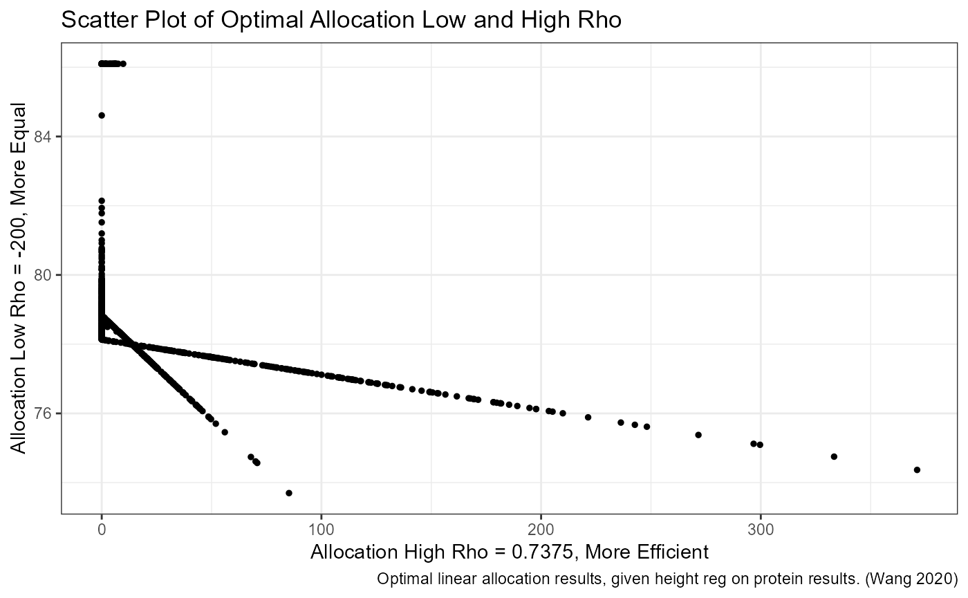
# lineplot <- tb_opti %>%
#     gather(variable, value, -month) %>%
#     ggplot(aes(x=month, y=value, colour=variable, linetype=variable)) +
#         geom_line() +
#         geom_point() +
#         labs(title = 'Mean and SD of Temperature Acorss US Cities',
#              x = 'Months',
#              y = 'Temperature in Fahrenheit',
#              caption = 'Temperature data 2017') +
#         scale_x_continuous(labels = as.character(df_temp_mth_summ$month),
#                            breaks = df_temp_mth_summ$month)