Logit Employment Binary Allocation Lalonde Training Example by Age Only
Source:vignettes/ffv_opt_sobin_rkone_allfc_training_logit_sub.Rmd
ffv_opt_sobin_rkone_allfc_training_logit_sub.RmdIn Logit Employment Binary Allocation Lalonde Training Example, analyzed optimal allocation when all observables attributes of individuals are used for targeting. Subgroup allocation targeting here, based on one attribute.
Set Up
Get Data
spt_img_save <- '../_img/'
spt_img_save_draft <- 'C:/Users/fan/Documents/Dropbox (UH-ECON)/repos/HgtOptiAlloDraft/_img/'
The regression is the same as prior. Subgroup allocation is based on the idea of targeting only a subset of individuals, when we know the marginal effects and needs of all individuals.
# Dataset
data(df_opt_lalonde_training)

# Add a binary variable for if there are wage in year 1975
dft <- df_opt_lalonde_training %>%
  mutate(re75_zero = case_when(re75 == 0 ~ 1, re75 != 0 ~ 0))

# dft stands for dataframe training
dft <- dft %>% mutate(id = X) %>%
           select(-X) %>%
           select(id, everything()) %>%
           mutate(emp78 =
                    case_when(re78 <= 0 ~ 0,
                              TRUE ~ 1)) %>%
           mutate(emp75 =
                    case_when(re75 <= 0 ~ 0,
                              TRUE ~ 1))

# Generate combine black + hispanic status
# 0 = white, 1 = black, 2 = hispanics
dft <- dft %>%
    mutate(race =
             case_when(black == 1 ~ 1,
                       hisp == 1 ~ 2,
                       TRUE ~ 0))

dft <- dft %>%
    mutate(age_m2 =
             case_when(age <= 23 ~ 1,
                       age >  23~ 2)) %>%
    mutate(age_m3 =
             case_when(age <= 20 ~ 1,
                       age > 20 & age <= 26 ~ 2,
                       age > 26 ~ 3))

dft$trt <- factor(dft$trt, levels = c(0,1), labels = c("ntran", "train"))

summary(dft)
## id trt age educ black
## Min. : 1.0 ntran:425 Min. :17.00 Min. : 3.00 Min. :0.0000
## 1st Qu.: 181.2 train:297 1st Qu.:19.00 1st Qu.: 9.00 1st Qu.:1.0000
## Median : 361.5 Median :23.00 Median :10.00 Median :1.0000
## Mean : 854.4 Mean :24.52 Mean :10.27 Mean :0.8006
## 3rd Qu.:1458.5 3rd Qu.:27.00 3rd Qu.:11.00 3rd Qu.:1.0000
## Max. :4110.0 Max. :55.00 Max. :16.00 Max. :1.0000
##
## hisp marr nodeg re74
## Min. :0.0000 Min. :0.000 Min. :0.0000 Min. : 0.0
## 1st Qu.:0.0000 1st Qu.:0.000 1st Qu.:1.0000 1st Qu.: 0.0
## Median :0.0000 Median :0.000 Median :1.0000 Median : 0.0
## Mean :0.1053 Mean :0.162 Mean :0.7798 Mean : 2102.3
## 3rd Qu.:0.0000 3rd Qu.:0.000 3rd Qu.:1.0000 3rd Qu.: 824.4
## Max. :1.0000 Max. :1.000 Max. :1.0000 Max. :39570.7
## NA's :277
## re75 re78 re75_zero emp78
## Min. : 0.0 Min. : 0 Min. :0.0000 Min. :0.0000
## 1st Qu.: 0.0 1st Qu.: 0 1st Qu.:0.0000 1st Qu.:0.0000
## Median : 936.3 Median : 3952 Median :0.0000 Median :1.0000
## Mean : 3042.9 Mean : 5455 Mean :0.4003 Mean :0.7285
## 3rd Qu.: 3993.2 3rd Qu.: 8772 3rd Qu.:1.0000 3rd Qu.:1.0000
## Max. :37431.7 Max. :60308 Max. :1.0000 Max. :1.0000
##
## emp75 race age_m2 age_m3
## Min. :0.0000 Min. :0.000 Min. :1.000 Min. :1.000
## 1st Qu.:0.0000 1st Qu.:1.000 1st Qu.:1.000 1st Qu.:1.000
## Median :1.0000 Median :1.000 Median :1.000 Median :2.000
## Mean :0.5997 Mean :1.011 Mean :1.486 Mean :1.965
## 3rd Qu.:1.0000 3rd Qu.:1.000 3rd Qu.:2.000 3rd Qu.:3.000
## Max. :1.0000 Max. :2.000 Max. :2.000 Max. :3.000
##
# X-variables to use on RHS
ls_st_xs <- c('age', 'educ',
              'black','hisp','marr', 'nodeg')
svr_binary <- 'trt'
svr_binary_lb0 <- 'ntran'
svr_binary_lb1 <- 'train'
svr_outcome <- 'emp78'
sdt_name <- 'NSW Lalonde Training'
Logit Regression
Prediction with Observed Binary Input
Logit regression with a continuous variable and a binary variable. Predict outcome with observed continuous variable as well as observed binary input variable.
# Regress No bivariate
rs_logit <- glm(as.formula(paste(svr_outcome,
                                 "~", paste(ls_st_xs, collapse="+")))
                ,data = dft, family = "binomial")
summary(rs_logit)
##
## Call:
## glm(formula = as.formula(paste(svr_outcome, "~", paste(ls_st_xs,
## collapse = "+"))), family = "binomial", data = dft)
##
## Deviance Residuals:
## Min 1Q Median 3Q Max
## -2.2075 -1.4253 0.7851 0.8571 1.1189
##
## Coefficients:
## Estimate Std. Error z value Pr(>|z|)
## (Intercept) 2.90493 0.99594 2.917 0.00354 **
## age -0.01870 0.01295 -1.445 0.14855
## educ -0.02754 0.06653 -0.414 0.67896
## black -1.16273 0.38941 -2.986 0.00283 **
## hisp -0.12130 0.51185 -0.237 0.81267
## marr 0.30300 0.24551 1.234 0.21714
## nodeg -0.29036 0.27833 -1.043 0.29684
## ---
## Signif. codes: 0 '***' 0.001 '**' 0.01 '*' 0.05 '.' 0.1 ' ' 1
##
## (Dispersion parameter for binomial family taken to be 1)
##
## Null deviance: 844.33 on 721 degrees of freedom
## Residual deviance: 818.46 on 715 degrees of freedom
## AIC: 832.46
##
## Number of Fisher Scoring iterations: 4
dft$p_mpg <- predict(rs_logit, newdata = dft, type = "response")

# Regress with bivariate
# rs_logit_bi <- glm(as.formula(paste(svr_outcome,
#                                     "~ factor(", svr_binary,") + ",
#                                     paste(ls_st_xs, collapse="+")))
#                    , data = dft, family = "binomial")
rs_logit_bi <- glm(emp78 ~
                     age + I(age^2) + factor(age_m2)
                   # + educ + I(educ^2) +
                   # + educ + black + hisp + marr + nodeg
                   + factor(trt)
                   + factor(age_m2)*factor(trt)
                   , data = dft, family = "binomial")
summary(rs_logit_bi)
##
## Call:
## glm(formula = emp78 ~ age + I(age^2) + factor(age_m2) + factor(trt) +
## factor(age_m2) * factor(trt), family = "binomial", data = dft)
##
## Deviance Residuals:
## Min 1Q Median 3Q Max
## -1.8735 -1.4565 0.7760 0.8054 0.9258
##
## Coefficients:
## Estimate Std. Error z value Pr(>|z|)
## (Intercept) 2.198320 1.620518 1.357 0.1749
## age -0.089819 0.116067 -0.774 0.4390
## I(age^2) 0.001409 0.001740 0.809 0.4183
## factor(age_m2)2 -0.141184 0.372152 -0.379 0.7044
## factor(trt)train 0.486634 0.257058 1.893 0.0583 .
## factor(age_m2)2:factor(trt)train -0.153539 0.351666 -0.437 0.6624
## ---
## Signif. codes: 0 '***' 0.001 '**' 0.01 '*' 0.05 '.' 0.1 ' ' 1
##
## (Dispersion parameter for binomial family taken to be 1)
##
## Null deviance: 844.33 on 721 degrees of freedom
## Residual deviance: 833.53 on 716 degrees of freedom
## AIC: 845.53
##
## Number of Fisher Scoring iterations: 4
# Predcit Using Regresion Data
dft$p_mpg_hp <- predict(rs_logit_bi, newdata = dft, type = "response")

# Predicted Probabilities am on mgp with or without hp binary
scatter <- ggplot(dft, aes(x=p_mpg_hp, y=p_mpg)) +
      geom_point(size=1) +
      # geom_smooth(method=lm) + # Trend line
      geom_abline(intercept = 0, slope = 1) + # 45 degree line
      labs(title = paste0('Predicted Probabilities ', svr_outcome, ' on ', ls_st_xs, ' with or without hp binary'),
           x = paste0('prediction with ', ls_st_xs, ' and binary ', svr_binary, ' indicator, 1 is high'),
           y = paste0('prediction with only ', ls_st_xs),
           caption = paste0(sdt_name, ' simulated prediction')) +
      theme_bw()
print(scatter)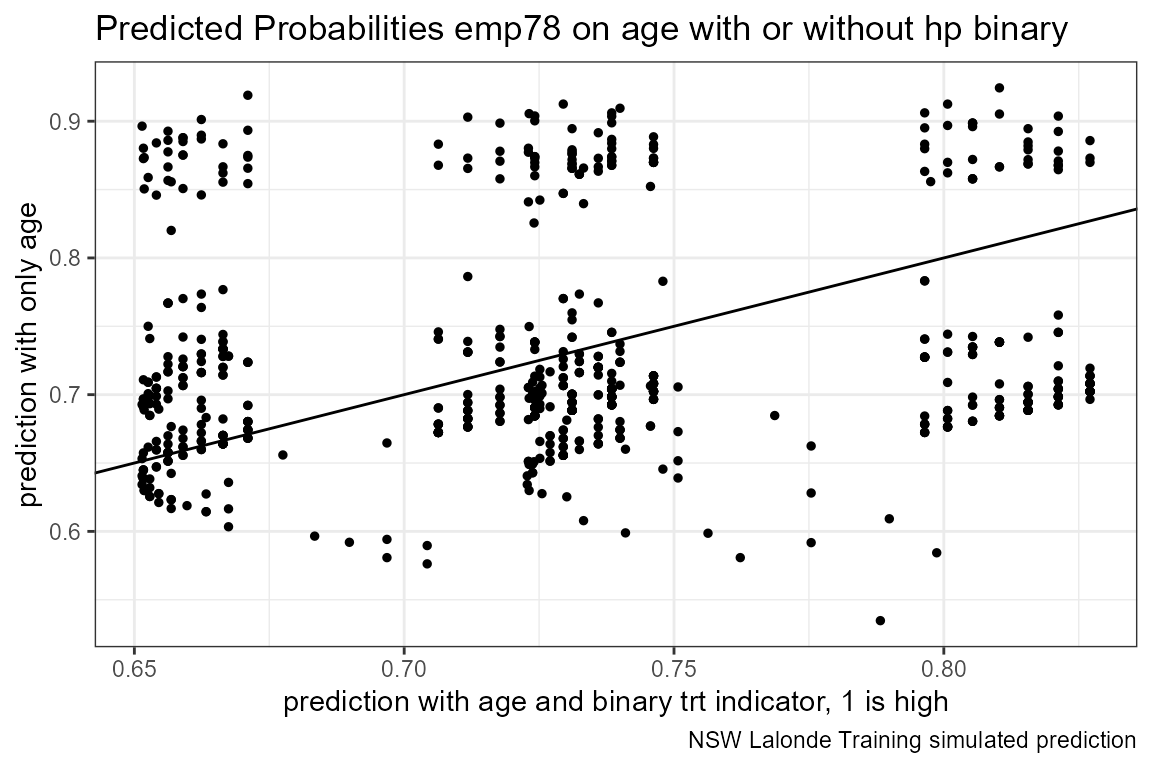
Prediction with Binary set to 0 and 1
Now generate two predictions. One set where binary input is equal to 0, and another where the binary inputs are equal to 1. Ignore whether in data binary input is equal to 0 or 1. Use the same regression results as what was just derived.
Note that given the example here, the probability changes a lot when we
# Previous regression results
summary(rs_logit_bi)
##
## Call:
## glm(formula = emp78 ~ age + I(age^2) + factor(age_m2) + factor(trt) +
## factor(age_m2) * factor(trt), family = "binomial", data = dft)
##
## Deviance Residuals:
## Min 1Q Median 3Q Max
## -1.8735 -1.4565 0.7760 0.8054 0.9258
##
## Coefficients:
## Estimate Std. Error z value Pr(>|z|)
## (Intercept) 2.198320 1.620518 1.357 0.1749
## age -0.089819 0.116067 -0.774 0.4390
## I(age^2) 0.001409 0.001740 0.809 0.4183
## factor(age_m2)2 -0.141184 0.372152 -0.379 0.7044
## factor(trt)train 0.486634 0.257058 1.893 0.0583 .
## factor(age_m2)2:factor(trt)train -0.153539 0.351666 -0.437 0.6624
## ---
## Signif. codes: 0 '***' 0.001 '**' 0.01 '*' 0.05 '.' 0.1 ' ' 1
##
## (Dispersion parameter for binomial family taken to be 1)
##
## Null deviance: 844.33 on 721 degrees of freedom
## Residual deviance: 833.53 on 716 degrees of freedom
## AIC: 845.53
##
## Number of Fisher Scoring iterations: 4
# Two different dataframes, mutate the binary regressor
dft_bi0 <- dft %>% mutate(!!sym(svr_binary) := svr_binary_lb0)
dft_bi1 <- dft %>% mutate(!!sym(svr_binary) := svr_binary_lb1)

# Predcit Using Regresion Data
dft$p_mpg_hp_bi0 <- predict(rs_logit_bi, newdata = dft_bi0, type = "response")
dft$p_mpg_hp_bi1 <- predict(rs_logit_bi, newdata = dft_bi1, type = "response")

# Predicted Probabilities and Binary Input
scatter <- ggplot(dft, aes(x=p_mpg_hp_bi0)) +
      geom_point(aes(y=p_mpg_hp), size=4, shape=4, color="red") +
      geom_point(aes(y=p_mpg_hp_bi1), size=2, shape=8) +
      # geom_smooth(method=lm) + # Trend line
      geom_abline(intercept = 0, slope = 1) + # 45 degree line
      labs(title = paste0('Predicted Probabilities and Binary Input',
                          '\ncross(shape=4)/red is predict actual binary data',
                          '\nstar(shape=8)/black is predict set binary = 1 for all'),
           x = paste0('prediction with ', ls_st_xs, ' and binary ', svr_binary, ' = 0 for all'),
           y = paste0('prediction with ', ls_st_xs, ' and binary ', svr_binary, ' = 1'),
           caption = paste0(sdt_name, ' simulated prediction')) +
      theme_bw()
print(scatter)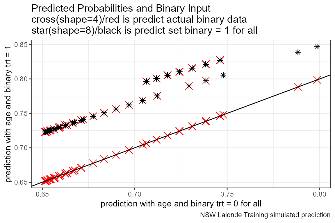
Generate and Analyze Individual A and alpha
Prediction with Binary set to 0 and 1 Difference
What is the difference in probability between binary = 0 vs binary = 1. How does that relate to the probability of outcome of interest when binary = 0 for all.
In the binary logit case, the relationship will be hump–shaped by construction between \(A_i\) and \(\alpha_i\). In the exponential wage cases, the relationship is convex upwards.
# Generate Gap Variable
dft <- dft %>% mutate(alpha_i = p_mpg_hp_bi1 - p_mpg_hp_bi0) %>%
                mutate(A_i = p_mpg_hp_bi0)

dft_graph <- dft
dft_graph$age_m2 <- factor(dft_graph$age_m2, labels = c('Age <= 23', 'Age > 23'))

# Titling
title_line1 <- sprintf("Each circle (cross) represents an individual <= age 23 (> age 23)")
title_line2 <- sprintf("Heterogeneous expected outcome (employment probability) with and without training")
title_line3 <- sprintf("Heterogeneity from logistic regression nonlinearity and heterogeneous age group effects")
title <- expression('The joint distribution of'~A[i]~'and'~alpha[i]~','~'Logistic Regression, Lalonde (AER, 1986)')
caption <- paste0('Logistic regression predictions of the employment effects of a training RCT. Data from Lalonde (AER, 1986).')
# Labels
st_x_label <- expression(A[i]~', '~Probability~of~Employment~without~Training~','~'P(train=0)')
st_y_label <- expression(alpha[i]~','~Marginal~Effects~of~Training~','~'P(train=1) - P(train=0)')

# Binary Marginal Effects and Prediction without Binary
plt_A_alpha <- dft_graph %>% ggplot(aes(x=A_i)) +
      geom_point(aes(y=alpha_i,
                     color=factor(age_m2),
                     shape=factor(age_m2)), size=4) +
      geom_abline(intercept = 0, slope = 1) + # 45 degree line
      scale_colour_manual(values=c("#69b3a2", "#404080")) +
      labs(subtitle = paste0(title_line1,'\n', title_line2, '\n', title_line3),
           x = st_x_label,
           y = st_y_label,
           caption = caption) +
      theme_bw(base_size=8) +
      scale_shape_manual(values=c(1, 4)) +
      guides(color=FALSE)
## Warning: `guides(<scale> = FALSE)` is deprecated. Please use `guides(<scale> =
## "none")` instead.
# Labeling
plt_A_alpha$labels$shape <- "Age Subgroups"

print(plt_A_alpha)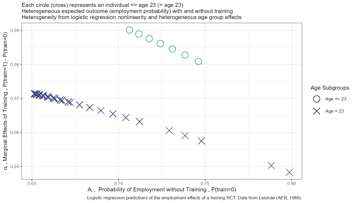
if (bl_save_img) {
  snm_cnts <- 'Lalonde_employ_A_alpha_age.png'
  png(paste0(spt_img_save, snm_cnts),
        width = 135, height = 86, units='mm', res = 300, pointsize=7)
  print(plt_A_alpha)
  dev.off()
  png(paste0(spt_img_save_draft, snm_cnts),
        width = 135, height = 86, units='mm', res = 300,
      pointsize=5)
  print(plt_A_alpha)
  dev.off()
}
Optimal Binary Allocation
Solve for Optimal Allocaions Across Preference Parameters
Invoke the binary optimal allocation function ffp_opt_anlyz_rhgin_bin that loops over rhos.
svr_inpalc <- 'rank'
dft <- cbind(dft, beta_i)
svr_rho_val <- 'rho_val'
ls_bin_solu_all_rhos <-
  ffp_opt_anlyz_rhgin_bin(dft, svr_id_i = 'id',
                          svr_A_i = 'A_i', svr_alpha_i = 'alpha_i', svr_beta_i = 'beta_i',
                          ar_rho = ar_rho,
                          svr_rho = 'rho', svr_rho_val = svr_rho_val,
                          svr_inpalc = svr_inpalc,
                          svr_expout = 'opti_exp_outcome',
                          verbose = TRUE)
## 'data.frame': 722 obs. of 54 variables:
## $ id : int 1 2 3 4 5 6 7 8 9 10 ...
## $ trt : Factor w/ 2 levels "ntran","train": 1 1 1 1 1 1 1 1 1 1 ...
## $ age : int 23 26 22 34 18 45 18 27 24 34 ...
## $ educ : int 10 12 9 9 9 11 9 12 8 11 ...
## $ black : int 1 0 1 1 1 1 1 1 0 1 ...
## $ hisp : int 0 0 0 0 0 0 0 0 0 0 ...
## $ marr : int 0 0 0 0 0 0 0 0 0 1 ...
## $ nodeg : int 1 0 1 1 1 1 1 0 1 1 ...
## $ re74 : num 0 0 0 NA 0 0 0 NA 0 0 ...
## $ re75 : num 0 0 0 4368 0 ...
## $ re78 : num 0 12384 0 14051 10740 ...
## $ re75_zero : num 1 1 1 0 1 1 1 0 1 1 ...
## $ emp78 : num 0 1 0 1 1 1 1 1 1 1 ...
## $ emp75 : num 0 0 0 1 0 0 0 1 0 0 ...
## $ race : num 1 0 1 1 1 1 1 1 0 1 ...
## $ age_m2 : num 1 2 1 2 1 2 1 2 2 2 ...
## $ age_m3 : num 2 2 2 3 1 3 1 3 2 3 ...
## $ p_mpg : num 0.678 0.89 0.688 0.638 0.704 ...
## $ p_mpg_hp : num 0.706 0.662 0.712 0.653 0.738 ...
## $ p_mpg_hp_bi0: num 0.706 0.662 0.712 0.653 0.738 ...
## $ p_mpg_hp_bi1: num 0.796 0.732 0.801 0.724 0.821 ...
## $ alpha_i : num 0.0901 0.0701 0.0889 0.0712 0.0828 ...
## $ A_i : num 0.706 0.662 0.712 0.653 0.738 ...
## $ beta_i : num 0.00139 0.00139 0.00139 0.00139 0.00139 ...
## $ rho_c1_rk : int 1 553 42 423 245 711 245 503 656 423 ...
## $ rho_c2_rk : int 1 553 42 423 245 711 245 503 656 423 ...
## $ rho_c3_rk : int 1 553 42 423 245 711 245 503 656 423 ...
## $ rho_c4_rk : int 1 553 42 423 245 711 245 503 656 423 ...
## $ rho_c5_rk : int 1 553 42 423 245 711 245 503 656 423 ...
## $ rho_c6_rk : int 1 553 42 423 245 711 245 503 656 423 ...
## $ rho_c7_rk : int 1 553 42 423 245 711 245 503 656 423 ...
## $ rho_c8_rk : int 1 553 42 423 245 711 245 503 656 423 ...
## $ rho_c9_rk : int 1 553 42 423 245 711 245 503 656 423 ...
## $ rho_c10_rk : int 1 553 42 423 245 711 245 503 656 423 ...
## $ rho_c11_rk : int 1 553 42 423 245 711 245 503 656 423 ...
## $ rho_c12_rk : int 1 553 42 423 245 711 245 503 656 423 ...
## $ rho_c13_rk : int 1 553 42 423 245 711 245 503 656 423 ...
## $ rho_c14_rk : int 1 553 42 423 245 711 245 503 656 423 ...
## $ rho_c15_rk : int 1 553 42 423 245 711 245 503 656 423 ...
## $ rho_c16_rk : int 1 553 42 371 252 711 252 451 656 371 ...
## $ rho_c17_rk : int 1 426 42 233 468 711 468 376 604 233 ...
## $ rho_c18_rk : int 1 305 42 135 573 711 573 255 529 135 ...
## $ rho_c19_rk : int 132 223 265 52 580 711 580 173 408 52 ...
## $ rho_c20_rk : int 285 182 365 52 584 659 584 132 326 52 ...
## $ rho_c21_rk : int 329 182 375 52 587 521 587 132 285 52 ...
## $ rho_c22_rk : int 334 182 377 52 590 463 590 132 285 52 ...
## $ rho_c23_rk : int 336 182 381 52 590 423 590 132 285 52 ...
## $ rho_c24_rk : int 340 182 384 52 591 381 591 132 285 52 ...
## $ rho_c25_rk : int 340 182 384 52 591 381 591 132 285 52 ...
## $ rho_c26_rk : int 343 182 384 52 591 340 591 132 285 52 ...
## $ rho_c27_rk : int 343 182 384 52 591 340 591 132 285 52 ...
## $ rho_c28_rk : int 343 182 384 52 591 340 591 132 285 52 ...
## $ rho_c29_rk : int 343 182 384 52 591 340 591 132 285 52 ...
## $ rho_c30_rk : int 343 182 384 52 591 340 591 132 285 52 ...## Joining, by = "id"
df_all_rho <- ls_bin_solu_all_rhos$df_all_rho
df_all_rho_long <- ls_bin_solu_all_rhos$df_all_rho_long

# How many people have different ranks across rhos
it_how_many_vary_rank <- sum(df_all_rho$rank_max - df_all_rho$rank_min)
it_how_many_vary_rank
## [1] -255976Change in Rank along rho
# get rank when wage rho = 1
df_all_rho_rho_c1 <- df_all_rho %>% select(id, rho_c1_rk)
# Merge
df_all_rho_long <- df_all_rho_long %>% mutate(rho = as.numeric(rho)) %>%
                      left_join(df_all_rho_rho_c1, by='id')
# Select subset to graph
df_rank_graph <- df_all_rho_long %>%
                    mutate(id = factor(id)) %>%
                    filter((id == 1) |  # utilitarian rank = 1
                           (id == 11) |  # utilitarian rank = 101
                           (id == 5)  |  # utilitarian rank = 201
                           (id == 205) |  # utilitarian rank = 301
                           (id == 42)|  # utilitarian rank = 401
                           (id == 8) |  # utilitarian rank = 501
                           (id == 31) |  # utilitarian rank = 601
                           (id == 134)   # utilitarian rank = 701
                           ) %>%
                    mutate(one_minus_rho = 1 - !!sym(svr_rho_val)) %>%
                    mutate(rho_c1_rk = factor(rho_c1_rk))

df_rank_graph$rho_c1_rk
## [1] 1 1 1 1 1 1 1 1 1 1 1 1 1 1 1 1 1 1
## [19] 1 1 1 1 1 1 1 1 1 1 1 1 245 245 245 245 245 245
## [37] 245 245 245 245 245 245 245 245 245 245 245 245 245 245 245 245 245 245
## [55] 245 245 245 245 245 245 503 503 503 503 503 503 503 503 503 503 503 503
## [73] 503 503 503 503 503 503 503 503 503 503 503 503 503 503 503 503 503 503
## [91] 124 124 124 124 124 124 124 124 124 124 124 124 124 124 124 124 124 124
## [109] 124 124 124 124 124 124 124 124 124 124 124 124 595 595 595 595 595 595
## [127] 595 595 595 595 595 595 595 595 595 595 595 595 595 595 595 595 595 595
## [145] 595 595 595 595 595 595 401 401 401 401 401 401 401 401 401 401 401 401
## [163] 401 401 401 401 401 401 401 401 401 401 401 401 401 401 401 401 401 401
## [181] 700 700 700 700 700 700 700 700 700 700 700 700 700 700 700 700 700 700
## [199] 700 700 700 700 700 700 700 700 700 700 700 700 320 320 320 320 320 320
## [217] 320 320 320 320 320 320 320 320 320 320 320 320 320 320 320 320 320 320
## [235] 320 320 320 320 320 320
## Levels: 1 124 245 320 401 503 595 700
df_rank_graph$id <- factor(df_rank_graph$rho_c1_rk,
                           labels = c('Rank= 1  ', #200
                                      'Rank= 124', #110
                                      'Rank= 245', #95
                                      'Rank= 320', #217
                                      'Rank= 411', #274
                                      'Rank= 503', #101
                                      'Rank= 595',
                                      'Rank= 700'
                                       ))

# x-labels
x.labels <- c('λ=0.99', 'λ=0.90', 'λ=0', 'λ=-10', 'λ=-100')
x.breaks <- c(0.01, 0.10, 1, 10, 100)

# title line 2
title_line1 <- sprintf("Optimal allocation queue vary λ, allocate using only AGE")
title_line2 <- sprintf("Colored lines = different individuals from the NSW training dataset")
title_line3 <- sprintf("Track ranking changes for eight individuals ranked 1, 101, ..., 701 at λ=0.99")

# Graph Results--Draw
line.plot <- df_rank_graph %>%
  ggplot(aes(x=one_minus_rho, y=!!sym(svr_inpalc),
             group=fct_rev(id),
             colour=fct_rev(id), size=2)) +
  # geom_line(aes(linetype =fct_rev(id)), size=0.75) +
  geom_line(size=0.5) +
  geom_vline(xintercept=c(1), linetype="dotted") +
  labs(subtitle = paste0(title_line1, '\n', title_line2, '\n', title_line3),
       x = 'log10 Rescale of λ, Log10(λ)\nλ=1 Utilitarian (Maximize Average), λ=-infty Rawlsian (Maximize Mininum)',
       y = 'Optimal Allocation Queue Rank (1=highest)',
       caption = 'Based on logistic regression of the employment effects of a training RCT. Data from Lalonde (AER, 1986).') +
  scale_x_continuous(trans='log10', labels = x.labels, breaks = x.breaks) +
  theme_bw(base_size=8)

# Labeling
line.plot$labels$colour <- "At λ=0.99, i's"

# Print
print(line.plot)
if (bl_save_img) {
  snm_cnts <- 'Lalonde_employ_rank_age.png'
  png(paste0(spt_img_save, snm_cnts),
        width = 135, height = 86, units='mm', res = 300, pointsize=7)
  print(line.plot)
  dev.off()
  png(paste0(spt_img_save_draft, snm_cnts),
        width = 135, height = 86, units='mm', res = 300,
      pointsize=5)
  print(line.plot)
  dev.off()
}
Save Results
# Change Variable names so that this can becombined with logit file later
df_all_rho <- df_all_rho %>% rename_at(vars(starts_with("rho_")), funs(str_replace(., "rk", "rk_empage")))
## Warning: `funs()` was deprecated in dplyr 0.8.0.
## Please use a list of either functions or lambdas:
##
## # Simple named list:
## list(mean = mean, median = median)
##
## # Auto named with `tibble::lst()`:
## tibble::lst(mean, median)
##
## # Using lambdas
## list(~ mean(., trim = .2), ~ median(., na.rm = TRUE))
## This warning is displayed once every 8 hours.
## Call `lifecycle::last_lifecycle_warnings()` to see where this warning was generated.
df_all_rho <- df_all_rho %>%
        rename(A_i_empage = A_i, alpha_i_empage = alpha_i, beta_i_empage = beta_i,
               rank_min_empage = rank_min, rank_max_empage = rank_max, avg_rank_empage = avg_rank)

# Save File
if (bl_save_rda) {
  df_opt_lalonde_training_empage <- df_all_rho
  usethis::use_data(df_opt_lalonde_training_empage, df_opt_lalonde_training_empage, overwrite = TRUE)
}
Binary Marginal Effects and Prediction without Binary
What is the relationship between ranking,
# ggplot.A.alpha.x <- function(svr_x, df,
#                              svr_alpha = 'alpha_i', svr_A = "A_i"){
#
#   scatter <- ggplot(df, aes(x=!!sym(svr_x))) +
#         geom_point(aes(y=alpha_i), size=4, shape=4, color="red") +
#         geom_point(aes(y=A_i), size=2, shape=8, color="blue") +
#         geom_abline(intercept = 0, slope = 1) + # 45 degree line
#         labs(title = paste0('A (blue) and alpha (red) vs x variables=', svr_x),
#              x = svr_x,
#              y = 'Probabilities',
#              caption = paste0(sdt_name, ' simulated prediction')) +
#         theme_bw()
#
# return(scatter)
# }