Line by Line Test Binary Allocation with Linear Regression
Source:vignettes/ffv_opt_sobin_rkone_allrw_car.Rmd
ffv_opt_sobin_rkone_allrw_car.RmdThe objective of this file is to solve the linear \(N_i\in{0,1}\) and \(H_i\) problem without invoking any functions.
File name ffv_opt_sobin_rkone_allrw:
- opt: optimal allocation project
- sobin: binary provision solution
- rkone: rank at one
- allrw: all code line by line raw original file
Algorithm Outline
Given \(N\) individuals, if each individual could or could not receive the provision, given finite resource, and common cost, if total resource avaible could finance input for \(M\) individuals, there would be \(\frac{N!}{(M-N)!\cdot N!)}\) number of possible choices. Even with 10 individuals,
- Solve unconstrained relative optimal allocation solutions from the continuous optimal allocation problem.
- Evaluate relative allocations when allocation for \(q\) is equal to \(1\)
- This generates a new function where the y-axis values show outcomes for each other individual when individual \(q\) allocation is at \(1\).
- Treat the \(m\) components of the function as slope and intercept, the \(q\) remaining component is the \(x\), for each individual, there is a unique \(x\)
- The randk order fully determin the sequence of provisions. This is similar to how rank order is determined in the continuous problem, with just a tiny difference of \(\alpha\) added in the numerator.
Load Packages and Data
Load Data
Generate four categories by initial height and mother’s education levels combinations.
# Load Data
tb_mtcars <- as_tibble(rownames_to_column(mtcars, var = "carname")) %>% rowid_to_column()
attach(tb_mtcars)
## The following object is masked from package:ggplot2:
##
## mpg
# Summarize
str(tb_mtcars)
## tibble [32 x 13] (S3: tbl_df/tbl/data.frame)
## $ rowid : int [1:32] 1 2 3 4 5 6 7 8 9 10 ...
## $ carname: chr [1:32] "Mazda RX4" "Mazda RX4 Wag" "Datsun 710" "Hornet 4 Drive" ...
## $ mpg : num [1:32] 21 21 22.8 21.4 18.7 18.1 14.3 24.4 22.8 19.2 ...
## $ cyl : num [1:32] 6 6 4 6 8 6 8 4 4 6 ...
## $ disp : num [1:32] 160 160 108 258 360 ...
## $ hp : num [1:32] 110 110 93 110 175 105 245 62 95 123 ...
## $ drat : num [1:32] 3.9 3.9 3.85 3.08 3.15 2.76 3.21 3.69 3.92 3.92 ...
## $ wt : num [1:32] 2.62 2.88 2.32 3.21 3.44 ...
## $ qsec : num [1:32] 16.5 17 18.6 19.4 17 ...
## $ vs : num [1:32] 0 0 1 1 0 1 0 1 1 1 ...
## $ am : num [1:32] 1 1 1 0 0 0 0 0 0 0 ...
## $ gear : num [1:32] 4 4 4 3 3 3 3 4 4 4 ...
## $ carb : num [1:32] 4 4 1 1 2 1 4 2 2 4 ...
summary(tb_mtcars)## rowid carname mpg cyl
## Min. : 1.00 Length:32 Min. :10.40 Min. :4.000
## 1st Qu.: 8.75 Class :character 1st Qu.:15.43 1st Qu.:4.000
## Median :16.50 Mode :character Median :19.20 Median :6.000
## Mean :16.50 Mean :20.09 Mean :6.188
## 3rd Qu.:24.25 3rd Qu.:22.80 3rd Qu.:8.000
## Max. :32.00 Max. :33.90 Max. :8.000
## disp hp drat wt
## Min. : 71.1 Min. : 52.0 Min. :2.760 Min. :1.513
## 1st Qu.:120.8 1st Qu.: 96.5 1st Qu.:3.080 1st Qu.:2.581
## Median :196.3 Median :123.0 Median :3.695 Median :3.325
## Mean :230.7 Mean :146.7 Mean :3.597 Mean :3.217
## 3rd Qu.:326.0 3rd Qu.:180.0 3rd Qu.:3.920 3rd Qu.:3.610
## Max. :472.0 Max. :335.0 Max. :4.930 Max. :5.424
## qsec vs am gear
## Min. :14.50 Min. :0.0000 Min. :0.0000 Min. :3.000
## 1st Qu.:16.89 1st Qu.:0.0000 1st Qu.:0.0000 1st Qu.:3.000
## Median :17.71 Median :0.0000 Median :0.0000 Median :4.000
## Mean :17.85 Mean :0.4375 Mean :0.4062 Mean :3.688
## 3rd Qu.:18.90 3rd Qu.:1.0000 3rd Qu.:1.0000 3rd Qu.:4.000
## Max. :22.90 Max. :1.0000 Max. :1.0000 Max. :5.000
## carb
## Min. :1.000
## 1st Qu.:2.000
## Median :2.000
## Mean :2.812
## 3rd Qu.:4.000
## Max. :8.000
# Generate Discrete Version of continuous variables
tb_mtcars <- tb_mtcars %>%
    mutate(wgtLowHigh = cut(wt,
                             breaks=c(-Inf, 3.1, Inf),
                             labels=c("LowWgt","HighWgt"))) %>%
    mutate(dratLowHigh = cut(drat,
                             breaks=c(-Inf, 3.59, Inf),
                             labels=c("lowRearAxleRatio","highRearAxleRatio")))

# Relabel some factors
tb_mtcars$vs <- factor(tb_mtcars$vs,
                        levels = c(0,1),
                        labels = c("engineVShaped", "engineStraight"))
tb_mtcars$am <- factor(tb_mtcars$am,
                        levels = c(0,1),
                        labels = c("automatic", "manual"))
Exploration
Tabulation
# tabulate
tb_mtcars %>%
  group_by(am, vs) %>%
  summarize(freq = n()) %>%
  pivot_wider(names_from = vs, values_from = freq)
## `summarise()` has grouped output by 'am'. You can override using the `.groups` argument.## # A tibble: 2 x 3
## # Groups: am [2]
## am engineVShaped engineStraight
## <fct> <int> <int>
## 1 automatic 12 7
## 2 manual 6 7Summarize all, conditional on shift status. am variable is Transmission (0 = automatic, 1 = manual):
# summarize all
REconTools::ff_summ_percentiles(tb_mtcars, bl_statsasrows = FALSE)
## Warning: `funs()` was deprecated in dplyr 0.8.0.
## Please use a list of either functions or lambdas:
##
## # Simple named list:
## list(mean = mean, median = median)
##
## # Auto named with `tibble::lst()`:
## tibble::lst(mean, median)
##
## # Using lambdas
## list(~ mean(., trim = .2), ~ median(., na.rm = TRUE))
## This warning is displayed once every 8 hours.
## Call `lifecycle::last_lifecycle_warnings()` to see where this warning was generated.## Warning: `as.tibble()` was deprecated in tibble 2.0.0.
## Please use `as_tibble()` instead.
## The signature and semantics have changed, see `?as_tibble`.
## This warning is displayed once every 8 hours.
## Call `lifecycle::last_lifecycle_warnings()` to see where this warning was generated.## Warning: attributes are not identical across measure variables;
## they will be dropped## # A tibble: 10 x 19
## var n unique NAobs ZEROobs mean sd cv min p01 p05 p10
## <chr> <dbl> <dbl> <dbl> <dbl> <dbl> <dbl> <dbl> <dbl> <dbl> <dbl> <dbl>
## 1 carb 32 6 0 0 2.81 1.62 0.574 1 1 1 1
## 2 cyl 32 3 0 0 6.19 1.79 0.289 4 4 4 4
## 3 disp 32 27 0 0 231. 124. 0.537 71.1 72.5 77.4 80.6
## 4 drat 32 22 0 0 3.60 0.535 0.149 2.76 2.76 2.85 3.01
## 5 gear 32 3 0 0 3.69 0.738 0.200 3 3 3 3
## 6 hp 32 22 0 0 147. 68.6 0.467 52 55.1 63.6 66
## 7 mpg 32 25 0 0 20.1 6.03 0.300 10.4 10.4 12.0 14.3
## 8 qsec 32 30 0 0 17.8 1.79 0.100 14.5 14.5 15.0 15.5
## 9 rowid 32 32 0 0 16.5 9.38 0.569 1 1.31 2.55 4.1
## 10 wt 32 29 0 0 3.22 0.978 0.304 1.51 1.54 1.74 1.96
## # ... with 7 more variables: p25 <dbl>, p50 <dbl>, p75 <dbl>, p90 <dbl>,
## # p95 <dbl>, p99 <dbl>, max <dbl>
# summarize auto transition
REconTools::ff_summ_percentiles(tb_mtcars %>% filter(am == 0), bl_statsasrows = FALSE)
## Warning in min(rowid, na.rm = TRUE): no non-missing arguments to min; returning
## Inf## Warning in min(mpg, na.rm = TRUE): no non-missing arguments to min; returning
## Inf## Warning in min(cyl, na.rm = TRUE): no non-missing arguments to min; returning
## Inf## Warning in min(disp, na.rm = TRUE): no non-missing arguments to min; returning
## Inf## Warning in min(hp, na.rm = TRUE): no non-missing arguments to min; returning Inf## Warning in min(drat, na.rm = TRUE): no non-missing arguments to min; returning
## Inf## Warning in min(wt, na.rm = TRUE): no non-missing arguments to min; returning Inf## Warning in min(qsec, na.rm = TRUE): no non-missing arguments to min; returning
## Inf## Warning in min(gear, na.rm = TRUE): no non-missing arguments to min; returning
## Inf## Warning in min(carb, na.rm = TRUE): no non-missing arguments to min; returning
## Inf## Warning in max(rowid, na.rm = TRUE): no non-missing arguments to max; returning
## -Inf## Warning in max(mpg, na.rm = TRUE): no non-missing arguments to max; returning
## -Inf## Warning in max(cyl, na.rm = TRUE): no non-missing arguments to max; returning
## -Inf## Warning in max(disp, na.rm = TRUE): no non-missing arguments to max; returning
## -Inf## Warning in max(hp, na.rm = TRUE): no non-missing arguments to max; returning
## -Inf## Warning in max(drat, na.rm = TRUE): no non-missing arguments to max; returning
## -Inf## Warning in max(wt, na.rm = TRUE): no non-missing arguments to max; returning
## -Inf## Warning in max(qsec, na.rm = TRUE): no non-missing arguments to max; returning
## -Inf## Warning in max(gear, na.rm = TRUE): no non-missing arguments to max; returning
## -Inf## Warning in max(carb, na.rm = TRUE): no non-missing arguments to max; returning
## -Inf## Warning: attributes are not identical across measure variables;
## they will be dropped## # A tibble: 10 x 19
## var n unique NAobs ZEROobs mean sd cv min p01 p05 p10
## <chr> <dbl> <dbl> <dbl> <dbl> <dbl> <dbl> <dbl> <dbl> <dbl> <dbl> <dbl>
## 1 carb 0 0 0 0 NaN NA NA Inf NA NA NA
## 2 cyl 0 0 0 0 NaN NA NA Inf NA NA NA
## 3 disp 0 0 0 0 NaN NA NA Inf NA NA NA
## 4 drat 0 0 0 0 NaN NA NA Inf NA NA NA
## 5 gear 0 0 0 0 NaN NA NA Inf NA NA NA
## 6 hp 0 0 0 0 NaN NA NA Inf NA NA NA
## 7 mpg 0 0 0 0 NaN NA NA Inf NA NA NA
## 8 qsec 0 0 0 0 NaN NA NA Inf NA NA NA
## 9 rowid 0 0 0 0 NaN NA NA Inf NA NA NA
## 10 wt 0 0 0 0 NaN NA NA Inf NA NA NA
## # ... with 7 more variables: p25 <dbl>, p50 <dbl>, p75 <dbl>, p90 <dbl>,
## # p95 <dbl>, p99 <dbl>, max <dbl>
# summarize manual transition
REconTools::ff_summ_percentiles(tb_mtcars %>% filter(am == 1), bl_statsasrows = FALSE)
## Warning in min(rowid, na.rm = TRUE): no non-missing arguments to min; returning
## Inf## Warning in min(mpg, na.rm = TRUE): no non-missing arguments to min; returning
## Inf## Warning in min(cyl, na.rm = TRUE): no non-missing arguments to min; returning
## Inf## Warning in min(disp, na.rm = TRUE): no non-missing arguments to min; returning
## Inf## Warning in min(hp, na.rm = TRUE): no non-missing arguments to min; returning Inf## Warning in min(drat, na.rm = TRUE): no non-missing arguments to min; returning
## Inf## Warning in min(wt, na.rm = TRUE): no non-missing arguments to min; returning Inf## Warning in min(qsec, na.rm = TRUE): no non-missing arguments to min; returning
## Inf## Warning in min(gear, na.rm = TRUE): no non-missing arguments to min; returning
## Inf## Warning in min(carb, na.rm = TRUE): no non-missing arguments to min; returning
## Inf## Warning in max(rowid, na.rm = TRUE): no non-missing arguments to max; returning
## -Inf## Warning in max(mpg, na.rm = TRUE): no non-missing arguments to max; returning
## -Inf## Warning in max(cyl, na.rm = TRUE): no non-missing arguments to max; returning
## -Inf## Warning in max(disp, na.rm = TRUE): no non-missing arguments to max; returning
## -Inf## Warning in max(hp, na.rm = TRUE): no non-missing arguments to max; returning
## -Inf## Warning in max(drat, na.rm = TRUE): no non-missing arguments to max; returning
## -Inf## Warning in max(wt, na.rm = TRUE): no non-missing arguments to max; returning
## -Inf## Warning in max(qsec, na.rm = TRUE): no non-missing arguments to max; returning
## -Inf## Warning in max(gear, na.rm = TRUE): no non-missing arguments to max; returning
## -Inf## Warning in max(carb, na.rm = TRUE): no non-missing arguments to max; returning
## -Inf## Warning: attributes are not identical across measure variables;
## they will be dropped## # A tibble: 10 x 19
## var n unique NAobs ZEROobs mean sd cv min p01 p05 p10
## <chr> <dbl> <dbl> <dbl> <dbl> <dbl> <dbl> <dbl> <dbl> <dbl> <dbl> <dbl>
## 1 carb 0 0 0 0 NaN NA NA Inf NA NA NA
## 2 cyl 0 0 0 0 NaN NA NA Inf NA NA NA
## 3 disp 0 0 0 0 NaN NA NA Inf NA NA NA
## 4 drat 0 0 0 0 NaN NA NA Inf NA NA NA
## 5 gear 0 0 0 0 NaN NA NA Inf NA NA NA
## 6 hp 0 0 0 0 NaN NA NA Inf NA NA NA
## 7 mpg 0 0 0 0 NaN NA NA Inf NA NA NA
## 8 qsec 0 0 0 0 NaN NA NA Inf NA NA NA
## 9 rowid 0 0 0 0 NaN NA NA Inf NA NA NA
## 10 wt 0 0 0 0 NaN NA NA Inf NA NA NA
## # ... with 7 more variables: p25 <dbl>, p50 <dbl>, p75 <dbl>, p90 <dbl>,
## # p95 <dbl>, p99 <dbl>, max <dbl>Exploration Regressions
# A. Regree MPG on horse power and binary if Manual or not (manual = 1)
# 1. more horse power less MPG
# 2. manual larger MPG
print(summary(lm(mpg ~ hp + wt + factor(am) - 1)))
##
## Call:
## lm(formula = mpg ~ hp + wt + factor(am) - 1)
##
## Residuals:
## Min 1Q Median 3Q Max
## -3.4221 -1.7924 -0.3788 1.2249 5.5317
##
## Coefficients:
## Estimate Std. Error t value Pr(>|t|)
## hp -0.037479 0.009605 -3.902 0.000546 ***
## wt -2.878575 0.904971 -3.181 0.003574 **
## factor(am)0 34.002875 2.642659 12.867 2.82e-13 ***
## factor(am)1 36.086585 1.736338 20.783 < 2e-16 ***
## ---
## Signif. codes: 0 '***' 0.001 '**' 0.01 '*' 0.05 '.' 0.1 ' ' 1
##
## Residual standard error: 2.538 on 28 degrees of freedom
## Multiple R-squared: 0.9872, Adjusted R-squared: 0.9853
## F-statistic: 538.2 on 4 and 28 DF, p-value: < 2.2e-16
# B. Also incorporate now engine shape, vs = 0 if v-shaped
print(summary(lm(mpg ~ hp + factor(am) - 1)))
##
## Call:
## lm(formula = mpg ~ hp + factor(am) - 1)
##
## Residuals:
## Min 1Q Median 3Q Max
## -4.3843 -2.2642 0.1366 1.6968 5.8657
##
## Coefficients:
## Estimate Std. Error t value Pr(>|t|)
## hp -0.058888 0.007857 -7.495 2.92e-08 ***
## factor(am)0 26.584914 1.425094 18.655 < 2e-16 ***
## factor(am)1 31.861999 1.282279 24.848 < 2e-16 ***
## ---
## Signif. codes: 0 '***' 0.001 '**' 0.01 '*' 0.05 '.' 0.1 ' ' 1
##
## Residual standard error: 2.909 on 29 degrees of freedom
## Multiple R-squared: 0.9825, Adjusted R-squared: 0.9807
## F-statistic: 543.4 on 3 and 29 DF, p-value: < 2.2e-16##
## Call:
## lm(formula = mpg ~ hp + carb + factor(am):factor(vs) - 1)
##
## Residuals:
## Min 1Q Median 3Q Max
## -5.6849 -1.6087 0.3848 1.7451 4.7693
##
## Coefficients:
## Estimate Std. Error t value Pr(>|t|)
## hp -0.03576 0.01509 -2.37 0.0255 *
## carb -0.47247 0.59770 -0.79 0.4364
## factor(am)0:factor(vs)0 23.44984 2.24649 10.44 8.61e-11 ***
## factor(am)1:factor(vs)0 28.42114 2.41540 11.77 6.47e-12 ***
## factor(am)0:factor(vs)1 25.40774 1.53403 16.56 2.48e-15 ***
## factor(am)1:factor(vs)1 31.92748 1.36324 23.42 < 2e-16 ***
## ---
## Signif. codes: 0 '***' 0.001 '**' 0.01 '*' 0.05 '.' 0.1 ' ' 1
##
## Residual standard error: 2.786 on 26 degrees of freedom
## Multiple R-squared: 0.9856, Adjusted R-squared: 0.9823
## F-statistic: 297.2 on 6 and 26 DF, p-value: < 2.2e-16##
## Call:
## lm(formula = mpg ~ hp + carb + factor(vs) + factor(am):factor(vs))
##
## Residuals:
## Min 1Q Median 3Q Max
## -5.6849 -1.6087 0.3848 1.7451 4.7693
##
## Coefficients:
## Estimate Std. Error t value Pr(>|t|)
## (Intercept) 23.44984 2.24649 10.438 8.61e-11 ***
## hp -0.03576 0.01509 -2.370 0.025501 *
## carb -0.47247 0.59770 -0.790 0.436401
## factor(vs)1 1.95790 1.70400 1.149 0.261016
## factor(vs)0:factor(am)1 4.97130 1.77299 2.804 0.009421 **
## factor(vs)1:factor(am)1 6.51974 1.52000 4.289 0.000219 ***
## ---
## Signif. codes: 0 '***' 0.001 '**' 0.01 '*' 0.05 '.' 0.1 ' ' 1
##
## Residual standard error: 2.786 on 26 degrees of freedom
## Multiple R-squared: 0.8208, Adjusted R-squared: 0.7864
## F-statistic: 23.82 on 5 and 26 DF, p-value: 6.045e-09Regression with Data and Construct Input Arrays
Regress MPG on Manual Transmission
# regress and store results
mt_model <- model.matrix(~ hp + qsec + factor(vs) + factor(am):factor(vs))
rs_mpg_on_auto = lm(mpg ~ mt_model - 1)
print(summary(rs_mpg_on_auto))
##
## Call:
## lm(formula = mpg ~ mt_model - 1)
##
## Residuals:
## Min 1Q Median 3Q Max
## -5.6941 -1.8361 0.4586 1.8845 4.9360
##
## Coefficients:
## Estimate Std. Error t value Pr(>|t|)
## mt_model(Intercept) 25.44102 12.07886 2.106 0.04499 *
## mt_modelhp -0.04526 0.01313 -3.447 0.00194 **
## mt_modelqsec -0.09350 0.60876 -0.154 0.87912
## mt_modelfactor(vs)1 1.79185 1.97040 0.909 0.37150
## mt_modelfactor(vs)0:factor(am)1 3.97068 1.68750 2.353 0.02647 *
## mt_modelfactor(vs)1:factor(am)1 6.53375 1.78571 3.659 0.00113 **
## ---
## Signif. codes: 0 '***' 0.001 '**' 0.01 '*' 0.05 '.' 0.1 ' ' 1
##
## Residual standard error: 2.818 on 26 degrees of freedom
## Multiple R-squared: 0.9853, Adjusted R-squared: 0.9819
## F-statistic: 290.4 on 6 and 26 DF, p-value: < 2.2e-16
rs_mpg_on_auto_tidy = tidy(rs_mpg_on_auto)
rs_mpg_on_auto_tidy
## # A tibble: 6 x 5
## term estimate std.error statistic p.value
## <chr> <dbl> <dbl> <dbl> <dbl>
## 1 mt_model(Intercept) 25.4 12.1 2.11 0.0450
## 2 mt_modelhp -0.0453 0.0131 -3.45 0.00194
## 3 mt_modelqsec -0.0935 0.609 -0.154 0.879
## 4 mt_modelfactor(vs)1 1.79 1.97 0.909 0.372
## 5 mt_modelfactor(vs)0:factor(am)1 3.97 1.69 2.35 0.0265
## 6 mt_modelfactor(vs)1:factor(am)1 6.53 1.79 3.66 0.00113Construct Input Arrays \(A_i\) and \(\alpha_i\)
Multiply coefficient vector by covariate matrix to generate A vector that is child/individual specific.
# Estimates Table
head(rs_mpg_on_auto_tidy, 6)
## # A tibble: 6 x 5
## term estimate std.error statistic p.value
## <chr> <dbl> <dbl> <dbl> <dbl>
## 1 mt_model(Intercept) 25.4 12.1 2.11 0.0450
## 2 mt_modelhp -0.0453 0.0131 -3.45 0.00194
## 3 mt_modelqsec -0.0935 0.609 -0.154 0.879
## 4 mt_modelfactor(vs)1 1.79 1.97 0.909 0.372
## 5 mt_modelfactor(vs)0:factor(am)1 3.97 1.69 2.35 0.0265
## 6 mt_modelfactor(vs)1:factor(am)1 6.53 1.79 3.66 0.00113
# Covariates
head(mt_model, 5)
## (Intercept) hp qsec factor(vs)1 factor(vs)0:factor(am)1
## 1 1 110 16.46 0 1
## 2 1 110 17.02 0 1
## 3 1 93 18.61 1 0
## 4 1 110 19.44 1 0
## 5 1 175 17.02 0 0
## factor(vs)1:factor(am)1
## 1 0
## 2 0
## 3 1
## 4 0
## 5 0
# Covariates coefficients from regression (including constant)
ar_fl_cova_esti <- as.matrix(rs_mpg_on_auto_tidy %>% filter(!str_detect(term, 'am')) %>% select(estimate))
ar_fl_main_esti <- as.matrix(rs_mpg_on_auto_tidy %>% filter(str_detect(term, 'am')) %>% select(estimate))
head(ar_fl_cova_esti, 5)
## estimate
## [1,] 25.44102224
## [2,] -0.04526124
## [3,] -0.09349849
## [4,] 1.79184516
head(ar_fl_main_esti, 5)## estimate
## [1,] 3.970683
## [2,] 6.533746
# Select Matrix subcomponents
mt_cova <- as.matrix(as_tibble(mt_model) %>% select(-contains("am")))
mt_intr <- model.matrix(~ factor(vs) - 1)

# Generate A_i, use mt_cova_wth_const
ar_A_m <- mt_cova %*% ar_fl_cova_esti
head(ar_A_m, 5)
## estimate
## [1,] 18.92330
## [2,] 18.87094
## [3,] 21.28357
## [4,] 20.43652
## [5,] 15.92896## estimate
## 1 3.970683
## 2 3.970683
## 3 6.533746
## 4 6.533746
## 5 3.970683Matrix with Required Inputs for Allocation
# Initate Dataframe that will store all estimates and optimal allocation relevant information
# combine identifying key information along with estimation A, alpha results
# note that we only need indi.id as key
mt_opti <- cbind(ar_alpha_m, ar_A_m, ar_beta_m)
ar_st_varnames <- c('alpha', 'A', 'beta')
df_esti_alpha_A_beta <- as_tibble(mt_opti) %>% rename_all(~c(ar_st_varnames))
## Warning: The `x` argument of `as_tibble.matrix()` must have unique column names if `.name_repair` is omitted as of tibble 2.0.0.
## Using compatibility `.name_repair`.
## This warning is displayed once every 8 hours.
## Call `lifecycle::last_lifecycle_warnings()` to see where this warning was generated.
tb_key_alpha_A_beta <- bind_cols(tb_mtcars, df_esti_alpha_A_beta) %>%
              select(one_of(c('rowid', 'carname', 'mpg', 'hp', 'qsec', 'vs', 'am', ar_st_varnames)))

# Unique beta, A, and alpha check
tb_opti_unique <- tb_key_alpha_A_beta %>% group_by(!!!syms(ar_st_varnames)) %>%
                    arrange(!!!syms(ar_st_varnames)) %>%
                    summarise(n_obs_group=n())
## `summarise()` has grouped output by 'alpha', 'A'. You can override using the `.groups` argument.
# Only include currently automatic cars
tb_key_alpha_A_beta <-tb_key_alpha_A_beta %>% filter(am == 'automatic')

# Show cars
head(tb_key_alpha_A_beta, 32)
## # A tibble: 19 x 10
## rowid carname mpg hp qsec vs am alpha A beta
## <int> <chr> <dbl> <dbl> <dbl> <fct> <fct> <dbl> <dbl> <dbl>
## 1 4 Hornet 4 Drive 21.4 110 19.4 engineS~ auto~ 6.53 20.4 0.0312
## 2 5 Hornet Sportabout 18.7 175 17.0 engineV~ auto~ 3.97 15.9 0.0312
## 3 6 Valiant 18.1 105 20.2 engineS~ auto~ 6.53 20.6 0.0312
## 4 7 Duster 360 14.3 245 15.8 engineV~ auto~ 3.97 12.9 0.0312
## 5 8 Merc 240D 24.4 62 20 engineS~ auto~ 6.53 22.6 0.0312
## 6 9 Merc 230 22.8 95 22.9 engineS~ auto~ 6.53 20.8 0.0312
## 7 10 Merc 280 19.2 123 18.3 engineS~ auto~ 6.53 20.0 0.0312
## 8 11 Merc 280C 17.8 123 18.9 engineS~ auto~ 6.53 19.9 0.0312
## 9 12 Merc 450SE 16.4 180 17.4 engineV~ auto~ 3.97 15.7 0.0312
## 10 13 Merc 450SL 17.3 180 17.6 engineV~ auto~ 3.97 15.6 0.0312
## 11 14 Merc 450SLC 15.2 180 18 engineV~ auto~ 3.97 15.6 0.0312
## 12 15 Cadillac Fleetwood 10.4 205 18.0 engineV~ auto~ 3.97 14.5 0.0312
## 13 16 Lincoln Continental 10.4 215 17.8 engineV~ auto~ 3.97 14.0 0.0312
## 14 17 Chrysler Imperial 14.7 230 17.4 engineV~ auto~ 3.97 13.4 0.0312
## 15 21 Toyota Corona 21.5 97 20.0 engineS~ auto~ 6.53 21.0 0.0312
## 16 22 Dodge Challenger 15.5 150 16.9 engineV~ auto~ 3.97 17.1 0.0312
## 17 23 AMC Javelin 15.2 150 17.3 engineV~ auto~ 3.97 17.0 0.0312
## 18 24 Camaro Z28 13.3 245 15.4 engineV~ auto~ 3.97 12.9 0.0312
## 19 25 Pontiac Firebird 19.2 175 17.0 engineV~ auto~ 3.97 15.9 0.0312Optimal Linear Allocations
Parameters for Optimal Allocation
# Child Count
it_obs = dim(tb_opti_unique)[1]

# Vector of Planner Preference
ar_rho <- 1 - (10^(c(seq(-0.5, 0.5, length.out=18))))
ar_rho <- unique(ar_rho)
print(ar_rho)
## [1] 0.68377223 0.63790416 0.58538304 0.52524386 0.45638164 0.37753112
## [7] 0.28724352 0.18385992 0.06548079 -0.07006896 -0.22527986 -0.40300372
## [13] -0.60650600 -0.83952580 -1.10634454 -1.41186470 -1.76169981 -2.16227766Optimal binary Allocation (CRS)
This also works with any CRS CES.
# Optimal Linear Equation

# Pull arrays out
ar_A <- tb_key_alpha_A_beta %>% pull(A)
ar_alpha <- tb_key_alpha_A_beta %>% pull(alpha)
ar_beta <- tb_key_alpha_A_beta %>% pull(beta)

# Define Function for each individual m, with hard coded arrays
# This function is a function in the R folder's ffp_opt_sobin.R file as well
ffi_binary_dplyrdo_func <- function(ls_row, fl_rho,
                                    bl_old=FALSE){
  # @param bl_old, weather to use old incorrect solution
  # hard coded inputs are:
  # 1, ar_A
  # 2, ar_alpha
  # 3, ar_beta
  # note follow https://fanwangecon.github.io/R4Econ/support/function/fs_applysapplymutate.html

  svr_A_i = 'A'
  svr_alpha_i = 'alpha'
  svr_beta_i = 'beta'

  fl_alpha <- ls_row[[svr_alpha_i]]
  fl_A <- ls_row[[svr_A_i]]
  fl_beta <- ls_row[[svr_beta_i]]

  ar_left <- (
              ((ar_A + ar_alpha)^fl_rho - (ar_A)^fl_rho)
              /
              ((fl_A + fl_alpha)^fl_rho - (fl_A)^fl_rho)
             )
  ar_right <- ((ar_beta)/(fl_beta))
  ar_rank_val <- ar_left*ar_right

  ar_bl_rank_val <- (ar_rank_val >= 1)

  # Note need the negative multiple in front of array
  ar_rank <- rank((-1)*ar_rank_val, ties.method='min')
  it_rank <- sum(ar_bl_rank_val)

  return(list(it_rank=it_rank,
              ar_rank=ar_rank,
              ar_rank_val=ar_rank_val))
  # return(it_rank)
}

ls_ranks <- ffi_binary_dplyrdo_func(tb_key_alpha_A_beta[2,], 0.1)
it_rank <- ls_ranks$it_rank
ar_rank <- ls_ranks$ar_rank
ar_rank_val <- ls_ranks$ar_rank_val

# accumulate allocation results
tb_opti_alloc_all_rho <- tb_key_alpha_A_beta

# A. First Loop over Planner Preference
# Generate Rank Order
for (it_rho_ctr in seq(1,length(ar_rho))) {
  rho = ar_rho[it_rho_ctr]

  tb_with_rank <- tb_key_alpha_A_beta %>%
    mutate(queue_rank = ffi_binary_dplyrdo_func(tb_key_alpha_A_beta[1,], rho)$ar_rank)

  # m. Keep for df collection individual key + optimal allocation
  # _on stands for optimal nutritional choices
  # _eh stands for expected height
  tb_opti_allocate_wth_key <- tb_with_rank %>% select(one_of('rowid','queue_rank')) %>%
                                rename(!!paste0('rho_c', it_rho_ctr, '_rk') := !!sym('queue_rank'))

  # n. merge optimal allocaiton results from different planner preference
  tb_opti_alloc_all_rho <- tb_opti_alloc_all_rho %>% left_join(tb_opti_allocate_wth_key, by='rowid')
}

# o. print results
print(summary(tb_opti_alloc_all_rho))
## rowid carname mpg hp
## Min. : 4.00 Length:19 Min. :10.40 Min. : 62.0
## 1st Qu.: 8.50 Class :character 1st Qu.:14.95 1st Qu.:116.5
## Median :13.00 Mode :character Median :17.30 Median :175.0
## Mean :13.79 Mean :17.15 Mean :160.3
## 3rd Qu.:19.00 3rd Qu.:19.20 3rd Qu.:192.5
## Max. :25.00 Max. :24.40 Max. :245.0
## qsec vs am alpha
## Min. :15.41 engineVShaped :12 automatic:19 Min. :3.971
## 1st Qu.:17.18 engineStraight: 7 manual : 0 1st Qu.:3.971
## Median :17.82 Median :3.971
## Mean :18.18 Mean :4.915
## 3rd Qu.:19.17 3rd Qu.:6.534
## Max. :22.90 Max. :6.534
## A beta rho_c1_rk rho_c2_rk rho_c3_rk
## Min. :12.87 Min. :0.03125 Min. : 1.0 Min. : 1.0 Min. : 1.0
## 1st Qu.:15.05 1st Qu.:0.03125 1st Qu.: 5.5 1st Qu.: 5.5 1st Qu.: 5.5
## Median :15.93 Median :0.03125 Median :10.0 Median :10.0 Median :10.0
## Mean :17.15 Mean :0.03125 Mean :10.0 Mean :10.0 Mean :10.0
## 3rd Qu.:20.20 3rd Qu.:0.03125 3rd Qu.:14.5 3rd Qu.:14.5 3rd Qu.:14.5
## Max. :22.56 Max. :0.03125 Max. :19.0 Max. :19.0 Max. :19.0
## rho_c4_rk rho_c5_rk rho_c6_rk rho_c7_rk rho_c8_rk
## Min. : 1.0 Min. : 1.0 Min. : 1.0 Min. : 1.0 Min. : 1.0
## 1st Qu.: 5.5 1st Qu.: 5.5 1st Qu.: 5.5 1st Qu.: 5.5 1st Qu.: 5.5
## Median :10.0 Median :10.0 Median :10.0 Median :10.0 Median :10.0
## Mean :10.0 Mean :10.0 Mean :10.0 Mean :10.0 Mean :10.0
## 3rd Qu.:14.5 3rd Qu.:14.5 3rd Qu.:14.5 3rd Qu.:14.5 3rd Qu.:14.5
## Max. :19.0 Max. :19.0 Max. :19.0 Max. :19.0 Max. :19.0
## rho_c9_rk rho_c10_rk rho_c11_rk rho_c12_rk rho_c13_rk
## Min. : 1.0 Min. : 1.0 Min. : 1.0 Min. : 1.0 Min. : 1.0
## 1st Qu.: 5.5 1st Qu.: 5.5 1st Qu.: 5.5 1st Qu.: 5.5 1st Qu.: 5.5
## Median :10.0 Median :10.0 Median :10.0 Median :10.0 Median :10.0
## Mean :10.0 Mean :10.0 Mean :10.0 Mean :10.0 Mean :10.0
## 3rd Qu.:14.5 3rd Qu.:14.5 3rd Qu.:14.5 3rd Qu.:14.5 3rd Qu.:14.5
## Max. :19.0 Max. :19.0 Max. :19.0 Max. :19.0 Max. :19.0
## rho_c14_rk rho_c15_rk rho_c16_rk rho_c17_rk rho_c18_rk
## Min. : 1.0 Min. : 1.0 Min. : 1.0 Min. : 1.0 Min. : 1.0
## 1st Qu.: 5.5 1st Qu.: 5.5 1st Qu.: 5.5 1st Qu.: 5.5 1st Qu.: 5.5
## Median :10.0 Median :10.0 Median :10.0 Median :10.0 Median :10.0
## Mean :10.0 Mean :10.0 Mean :10.0 Mean :10.0 Mean :10.0
## 3rd Qu.:14.5 3rd Qu.:14.5 3rd Qu.:14.5 3rd Qu.:14.5 3rd Qu.:14.5
## Max. :19.0 Max. :19.0 Max. :19.0 Max. :19.0 Max. :19.0
str(tb_opti_alloc_all_rho)## tibble [19 x 28] (S3: tbl_df/tbl/data.frame)
## $ rowid : int [1:19] 4 5 6 7 8 9 10 11 12 13 ...
## $ carname : chr [1:19] "Hornet 4 Drive" "Hornet Sportabout" "Valiant" "Duster 360" ...
## $ mpg : num [1:19] 21.4 18.7 18.1 14.3 24.4 22.8 19.2 17.8 16.4 17.3 ...
## $ hp : num [1:19] 110 175 105 245 62 95 123 123 180 180 ...
## $ qsec : num [1:19] 19.4 17 20.2 15.8 20 ...
## $ vs : Factor w/ 2 levels "engineVShaped",..: 2 1 2 1 2 2 2 2 1 1 ...
## $ am : Factor w/ 2 levels "automatic","manual": 1 1 1 1 1 1 1 1 1 1 ...
## $ alpha : num [1:19] 6.53 3.97 6.53 3.97 6.53 ...
## $ A : num [1:19] 20.4 15.9 20.6 12.9 22.6 ...
## $ beta : num [1:19] 0.0312 0.0312 0.0312 0.0312 0.0312 ...
## $ rho_c1_rk : int [1:19] 3 17 4 8 7 5 2 1 15 14 ...
## $ rho_c2_rk : int [1:19] 3 17 4 8 7 5 2 1 15 14 ...
## $ rho_c3_rk : int [1:19] 3 17 4 8 7 5 2 1 15 14 ...
## $ rho_c4_rk : int [1:19] 3 17 4 8 7 5 2 1 15 14 ...
## $ rho_c5_rk : int [1:19] 3 17 4 8 7 5 2 1 15 14 ...
## $ rho_c6_rk : int [1:19] 3 17 4 8 7 5 2 1 15 14 ...
## $ rho_c7_rk : int [1:19] 3 17 4 8 7 5 2 1 15 14 ...
## $ rho_c8_rk : int [1:19] 3 17 4 8 7 5 2 1 15 14 ...
## $ rho_c9_rk : int [1:19] 3 17 4 7 9 5 2 1 15 14 ...
## $ rho_c10_rk: int [1:19] 4 17 6 3 11 7 2 1 15 14 ...
## $ rho_c11_rk: int [1:19] 6 17 7 1 12 8 5 4 15 14 ...
## $ rho_c12_rk: int [1:19] 8 16 9 1 17 10 6 5 14 13 ...
## $ rho_c13_rk: int [1:19] 8 16 9 1 17 11 7 6 13 12 ...
## $ rho_c14_rk: int [1:19] 13 12 14 1 19 15 10 7 9 8 ...
## $ rho_c15_rk: int [1:19] 13 10 14 1 19 15 12 11 8 7 ...
## $ rho_c16_rk: int [1:19] 15 10 16 1 19 17 12 11 8 7 ...
## $ rho_c17_rk: int [1:19] 15 10 16 1 19 17 14 13 8 7 ...
## $ rho_c18_rk: int [1:19] 15 10 16 1 19 17 14 13 8 7 ...
# Make Longer
st_bisec_prefix <- 'rho_c'
svr_abfafb_long_name <- 'rho'
svr_bisect_iter <- 'nothing'
svr_number_col <- 'rank'
  tb_opti_alloc_all_rho_long <- tb_opti_alloc_all_rho %>%
  pivot_longer(
    cols = starts_with(st_bisec_prefix),
    names_to = c(svr_abfafb_long_name, svr_bisect_iter),
    names_pattern = paste0(st_bisec_prefix, "(.*)_(.*)"),
    values_to = svr_number_col
  )

# rho as numeric
tb_opti_alloc_all_rho_long <- tb_opti_alloc_all_rho_long %>% mutate(rho_num = as.numeric(rho))
print(summary(tb_opti_alloc_all_rho_long))
## rowid carname mpg hp
## Min. : 4.00 Length:342 Min. :10.40 Min. : 62.0
## 1st Qu.: 8.00 Class :character 1st Qu.:14.70 1st Qu.:110.0
## Median :13.00 Mode :character Median :17.30 Median :175.0
## Mean :13.79 Mean :17.15 Mean :160.3
## 3rd Qu.:21.00 3rd Qu.:19.20 3rd Qu.:205.0
## Max. :25.00 Max. :24.40 Max. :245.0
## qsec vs am alpha
## Min. :15.41 engineVShaped :216 automatic:342 Min. :3.971
## 1st Qu.:17.05 engineStraight:126 manual : 0 1st Qu.:3.971
## Median :17.82 Median :3.971
## Mean :18.18 Mean :4.915
## 3rd Qu.:19.44 3rd Qu.:6.534
## Max. :22.90 Max. :6.534
## A beta rho nothing
## Min. :12.87 Min. :0.03125 Length:342 Length:342
## 1st Qu.:14.48 1st Qu.:0.03125 Class :character Class :character
## Median :15.93 Median :0.03125 Mode :character Mode :character
## Mean :17.15 Mean :0.03125
## 3rd Qu.:20.44 3rd Qu.:0.03125
## Max. :22.56 Max. :0.03125
## rank rho_num
## Min. : 1 Min. : 1.0
## 1st Qu.: 5 1st Qu.: 5.0
## Median :10 Median : 9.5
## Mean :10 Mean : 9.5
## 3rd Qu.:15 3rd Qu.:14.0
## Max. :19 Max. :18.0
str(tb_opti_alloc_all_rho_long)## tibble [342 x 14] (S3: tbl_df/tbl/data.frame)
## $ rowid : int [1:342] 4 4 4 4 4 4 4 4 4 4 ...
## $ carname: chr [1:342] "Hornet 4 Drive" "Hornet 4 Drive" "Hornet 4 Drive" "Hornet 4 Drive" ...
## $ mpg : num [1:342] 21.4 21.4 21.4 21.4 21.4 21.4 21.4 21.4 21.4 21.4 ...
## $ hp : num [1:342] 110 110 110 110 110 110 110 110 110 110 ...
## $ qsec : num [1:342] 19.4 19.4 19.4 19.4 19.4 ...
## $ vs : Factor w/ 2 levels "engineVShaped",..: 2 2 2 2 2 2 2 2 2 2 ...
## $ am : Factor w/ 2 levels "automatic","manual": 1 1 1 1 1 1 1 1 1 1 ...
## $ alpha : num [1:342] 6.53 6.53 6.53 6.53 6.53 ...
## $ A : num [1:342] 20.4 20.4 20.4 20.4 20.4 ...
## $ beta : num [1:342] 0.0312 0.0312 0.0312 0.0312 0.0312 ...
## $ rho : chr [1:342] "1" "2" "3" "4" ...
## $ nothing: chr [1:342] "rk" "rk" "rk" "rk" ...
## $ rank : int [1:342] 3 3 3 3 3 3 3 3 3 4 ...
## $ rho_num: num [1:342] 1 2 3 4 5 6 7 8 9 10 ...Bump Plot for Optimal Binary Allocations
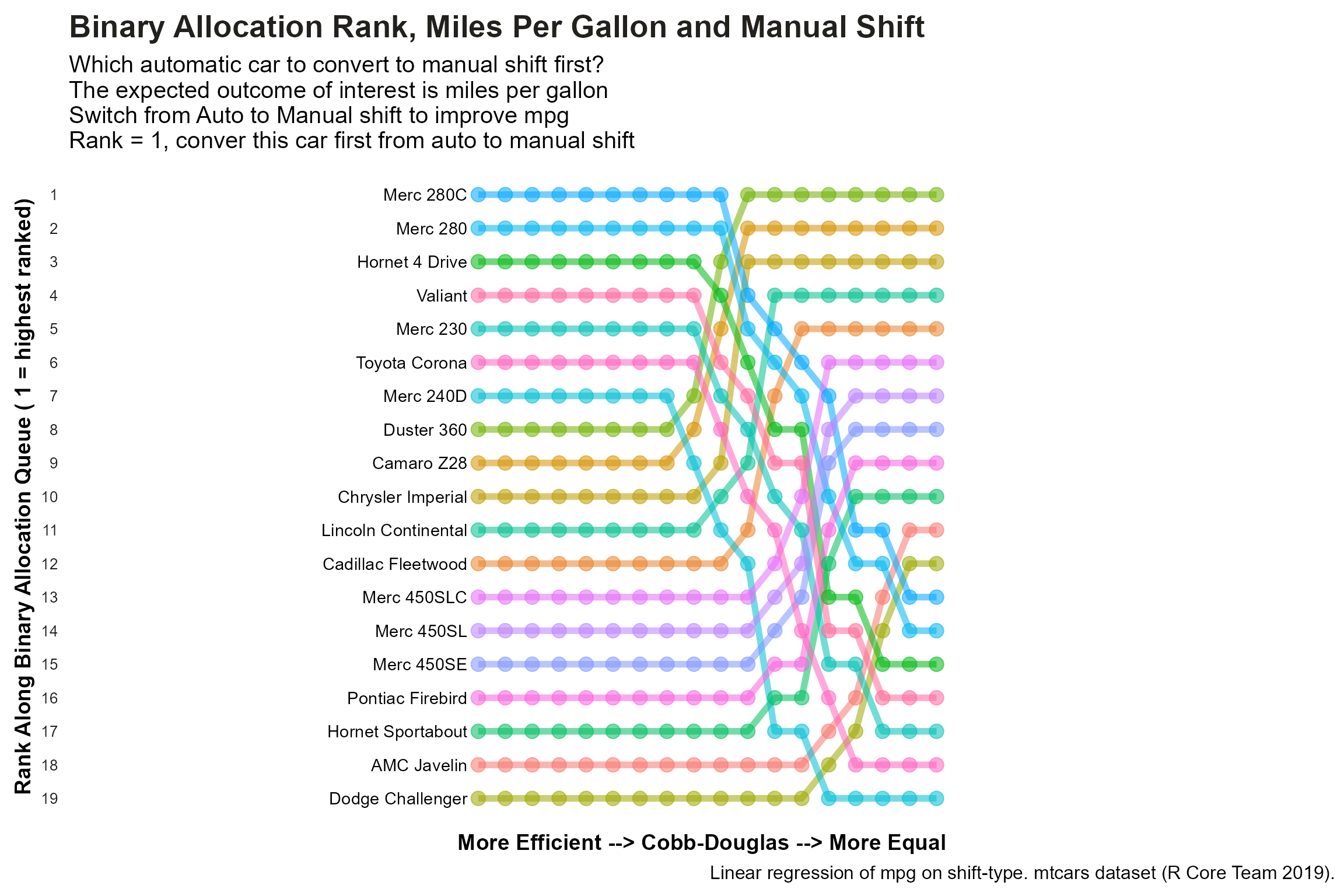
st_title = paste0("Binary Allocation Rank, Miles Per Gallon and Manual Shift")
st_subtitle = paste0("Which automatic car to convert to manual shift first?\n",
                     "The expected outcome of interest is miles per gallon\n",
                     "Switch from Auto to Manual shift to improve mpg\n",
                     "Rank = 1, conver this car first from auto to manual shift")
st_caption = paste0("Linear regression of mpg on shift-type. mtcars dataset (R Core Team 2019).")
st_x_lab = paste0("More Efficient --> Cobb-Douglas --> More Equal")
st_y_lab = paste0("Rank Along Binary Allocation Queue ( 1 = highest ranked)")

tb_opti_alloc_all_rho_long %>%
  ggplot(aes(x = rho_num, y = rank, group = carname)) +
    geom_line(aes(color = carname, alpha = 1), size = 2) +
    geom_point(aes(color = carname, alpha = 1), size = 4) +
    scale_x_discrete(expand = c(0.85,0))+
    scale_y_reverse(breaks = 1:nrow(tb_opti_alloc_all_rho_long))+
    theme(legend.position = "none") +
    labs(x = st_x_lab,
         y = st_y_lab,
         title = st_title,
         subtitle = st_subtitle,
         caption = st_caption) +
    ffy_opt_ghthm_dk() +
    geom_text(data = tb_opti_alloc_all_rho, aes(y=rho_c1_rk, x=0.6, label=carname),hjust="right")