Line by Line Test Log Linear Allocation Test
Source:vignettes/ffv_opt_solog_bisec_allrw.Rmd
ffv_opt_solog_bisec_allrw.RmdGiven allocation space parameters (A, alpha) for log linear regression, test log-linear optima allocation line by line. The result is not included in the final version of the paper, because the results are not closed-form, but are based on a root search. The root search is very fast when initial condition is zero.
The objective of this file is to solve the log linear \(N_i\) and \(H_i\) problem without invoking any functions using bisection with the implicit solution derived in the paper.
File name ffv_opt_solog_bisec_allrw:
- opt: optimal allocation project
- solog: log linear production function
- bisec: implicit formula solved via bisection
- allrw: all code line by line raw original file
Input and Output
There is a dataset with child attributes, nutritional inputs and outputs. Run regression to estimate some input output relationship first. Then generate required inputs for code.
- Required Input
- @param df tibble data table including variables using svr names below each row is potentially an individual who will receive alternative allocations
- @param svr_A_i string name of the A_i variable, dot product of covariates and coefficients, TFP from log linear
- @param svr_alpha_i string name of the alpha_i variable, individual specific elasticity information, elasticity from log linear
- @param svr_beta_i string name of the beta_i variable, relative preference weight for each child
- @param svr_N_i string name of the vector of existing inputs, based on which to compute aggregate resource
- @param fl_N_hat float total resource avaible for allocation, if not specific, sum by svr_N_i
- @param fl_rho float preference for equality for the planner
- @return a dataframe that expands the df inputs with additional results, including bisection solution.
- The structure assumes some regression has already taken place to generate the i specific variables listed.
Load Packages and Data
common parameters
some important shared, common fixed parameters specify them here:
# which params to test
it_test = 6

# parameters
fl_rho = 0.20
svr_id_var = 'indi_id'

# it_child_count = n, the number of children
it_n_child_cnt = 2
# it_heter_param = q, number of parameters that are heterogeneous across children
it_q_hetpa_cnt = 2

# choice grid for nutritional feasible choices for each
fl_n_agg = 100
fl_n_min = 0
it_n_choice_cnt_ttest = 3
it_n_choice_cnt_dense = 100
a and alpha input matrix
different types of alpha and a combinations. the algorithm, solutions should work for any alpha and a.
if (it_test == 1) {
  # A. test params 1
  # these are initially what i tested with, positively correlated a and alpha, some have both higher tfp as well as elasticity.
  ar_nn_a = seq(-2, 2, length.out = it_n_child_cnt)
  ar_nn_alpha = seq(0.1, 0.9, length.out = it_n_child_cnt)
  mt_nn_by_nq_a_alpha = cbind(ar_nn_a, ar_nn_alpha)
} else if (it_test == 2) {
  # B. test params 2
  ar_nn_a = c(0,0)
  ar_nn_alpha = c(0.1,0.2)
  mt_nn_by_nq_a_alpha = cbind(ar_nn_a, ar_nn_alpha)
} else if (it_test == 3) {
  # C. test params 3
  ar_nn_a = c(0,0)
  ar_nn_alpha = c(0.1,0.1)
  mt_nn_by_nq_a_alpha = cbind(ar_nn_a, ar_nn_alpha)
} else if (it_test == 4) {
  # D. test params 4
  ar_nn_a = c(0,0)
  ar_nn_alpha = c(0.006686704,0.009251407)
  mt_nn_by_nq_a_alpha = cbind(ar_nn_a, ar_nn_alpha)
} else if (it_test == 5) {
  # E. test params 5
  ar_nn_a = c(4.342501, 4.359987)
  ar_nn_alpha = c(0.006686704,0.009251407)
  mt_nn_by_nq_a_alpha = cbind(ar_nn_a, ar_nn_alpha)
} else if (it_test == 6) {
  # graph b
  # input group two, from the project
  ls_opti_alpha_a <- ffy_opt_dtgch_cbem4()
  df_esti <- ls_opti_alpha_a$df_esti
  df_dtgch_cbem4_bisec <- df_esti[, c('A_log', 'alpha_log')]
  ar_nn_a <- df_dtgch_cbem4_bisec %>% pull(A_log)
  ar_nn_alpha <- df_dtgch_cbem4_bisec %>% pull(alpha_log)
  mt_nn_by_nq_a_alpha = cbind(ar_nn_a, ar_nn_alpha)
}
## Warning: The `x` argument of `as_tibble.matrix()` must have unique column names if `.name_repair` is omitted as of tibble 2.0.0.
## Using compatibility `.name_repair`.
## This warning is displayed once every 8 hours.
## Call `lifecycle::last_lifecycle_warnings()` to see where this warning was generated.expand matrix
# choice grid for nutritional feasible choices for each
it_n_choice_cnt_ttest = 3
it_n_choice_cnt_dense = 100
ar_n_choices_ttest = seq(fl_n_min, fl_n_agg, length.out = it_n_choice_cnt_ttest)
ar_n_choices_dense = seq(fl_n_min, fl_n_agg, length.out = it_n_choice_cnt_dense)

# mesh expand
tb_states_choices <- as_tibble(mt_nn_by_nq_a_alpha) %>% rowid_to_column(var=svr_id_var)
tb_states_choices_ttest <- tb_states_choices %>% sample_n(9, replace = FALSE) %>%
                              expand_grid(choices = ar_n_choices_ttest)
tb_states_choices_dense <- tb_states_choices %>% sample_n(9, replace = FALSE) %>%
                              expand_grid(choices = ar_n_choices_dense)

# display
summary(tb_states_choices_dense)
## indi_id ar_nn_a ar_nn_alpha choices
## Min. : 96.0 Min. :4.304 Min. :0.006687 Min. : 0
## 1st Qu.:231.0 1st Qu.:4.321 1st Qu.:0.006687 1st Qu.: 25
## Median :378.0 Median :4.331 Median :0.006687 Median : 50
## Mean :492.8 Mean :4.332 Mean :0.008172 Mean : 50
## 3rd Qu.:720.0 3rd Qu.:4.334 3rd Qu.:0.009251 3rd Qu.: 75
## Max. :920.0 Max. :4.372 Max. :0.012090 Max. :100
kable(tb_states_choices_ttest) %>%
kable_styling(bootstrap_options = c("striped", "hover", "condensed", "responsive"))| indi_id | ar_nn_a | ar_nn_alpha | choices |
|---|---|---|---|
| 299 | 4.326523 | 0.0066867 | 0 |
| 299 | 4.326523 | 0.0066867 | 50 |
| 299 | 4.326523 | 0.0066867 | 100 |
| 637 | 4.325891 | 0.0066867 | 0 |
| 637 | 4.325891 | 0.0066867 | 50 |
| 637 | 4.325891 | 0.0066867 | 100 |
| 615 | 4.366037 | 0.0139396 | 0 |
| 615 | 4.366037 | 0.0139396 | 50 |
| 615 | 4.366037 | 0.0139396 | 100 |
| 305 | 4.341420 | 0.0120902 | 0 |
| 305 | 4.341420 | 0.0120902 | 50 |
| 305 | 4.341420 | 0.0120902 | 100 |
| 677 | 4.364739 | 0.0139396 | 0 |
| 677 | 4.364739 | 0.0139396 | 50 |
| 677 | 4.364739 | 0.0139396 | 100 |
| 690 | 4.350469 | 0.0139396 | 0 |
| 690 | 4.350469 | 0.0139396 | 50 |
| 690 | 4.350469 | 0.0139396 | 100 |
| 657 | 4.342073 | 0.0066867 | 0 |
| 657 | 4.342073 | 0.0066867 | 50 |
| 657 | 4.342073 | 0.0066867 | 100 |
| 707 | 4.331892 | 0.0120902 | 0 |
| 707 | 4.331892 | 0.0120902 | 50 |
| 707 | 4.331892 | 0.0120902 | 100 |
| 856 | 4.347273 | 0.0066867 | 0 |
| 856 | 4.347273 | 0.0066867 | 50 |
| 856 | 4.347273 | 0.0066867 | 100 |
Apply Same Function All Rows, some inputs row-specific, other shared
3 points and denser dataframs and define function
# convert matrix to tibble
ar_st_col_names = c(svr_id_var,'fl_a', 'fl_alpha')
tb_states_choices <- tb_states_choices %>% rename_all(~c(ar_st_col_names))
ar_st_col_names = c(svr_id_var,'fl_a', 'fl_alpha', 'fl_n')
tb_states_choices_ttest <- tb_states_choices_ttest %>% rename_all(~c(ar_st_col_names))
tb_states_choices_dense <- tb_states_choices_dense %>% rename_all(~c(ar_st_col_names))

# define implicit function
ffi_nonlin_dplyrdo <- function(fl_a, fl_alpha, fl_n, ar_a, ar_alpha, fl_n_agg, fl_rho){
  # scalar value that are row-specific, in dataframe already: *fl_a*, *fl_alpha*, *fl_n*
  # array and scalars not in dataframe, common all rows: *ar_a*, *ar_alpha*, *fl_n_agg*, *fl_rho*

  # test parameters
  # ar_a = ar_nn_a
  # ar_alpha = ar_nn_alpha
  # fl_n = 100
  # fl_rho = -1
  # fl_n_q = 10

  # apply function
  ar_p1_s1 = exp((fl_a - ar_a)*fl_rho)
  ar_p1_s2 = (fl_alpha/ar_alpha)
  ar_p1_s3 = (1/(ar_alpha*fl_rho - 1))
  ar_p1 = (ar_p1_s1*ar_p1_s2)^ar_p1_s3
  ar_p2 = fl_n^((fl_alpha*fl_rho-1)/(ar_alpha*fl_rho-1))
  ar_overall = ar_p1*ar_p2
  fl_overall = fl_n_agg - sum(ar_overall)

  return(fl_overall)
}
evaluate at three choice points and show table
in the example below, just show results evaluating over three choice points and show table.
# fl_a, fl_alpha are from columns of tb_nn_by_nq_a_alpha
tb_states_choices_ttest_eval = tb_states_choices_ttest %>% rowwise() %>%
                        mutate(dplyr_eval = ffi_nonlin_dplyrdo(fl_a, fl_alpha, fl_n,
                                                               ar_nn_a, ar_nn_alpha,
                                                               fl_n_agg, fl_rho))
# show
kable(tb_states_choices_ttest_eval) %>%
kable_styling(bootstrap_options = c("striped", "hover", "condensed", "responsive"))| indi_id | fl_a | fl_alpha | fl_n | dplyr_eval |
|---|---|---|---|---|
| 299 | 4.326523 | 0.0066867 | 0 | 100.00 |
| 299 | 4.326523 | 0.0066867 | 50 | -81070.60 |
| 299 | 4.326523 | 0.0066867 | 100 | -162341.95 |
| 637 | 4.325891 | 0.0066867 | 0 | 100.00 |
| 637 | 4.325891 | 0.0066867 | 50 | -81080.90 |
| 637 | 4.325891 | 0.0066867 | 100 | -162362.56 |
| 615 | 4.366037 | 0.0139396 | 0 | 100.00 |
| 615 | 4.366037 | 0.0139396 | 50 | -38247.67 |
| 615 | 4.366037 | 0.0139396 | 100 | -76565.63 |
| 305 | 4.341420 | 0.0120902 | 0 | 100.00 |
| 305 | 4.341420 | 0.0120902 | 50 | -44410.91 |
| 305 | 4.341420 | 0.0120902 | 100 | -88910.21 |
| 677 | 4.364739 | 0.0139396 | 0 | 100.00 |
| 677 | 4.364739 | 0.0139396 | 50 | -38257.65 |
| 677 | 4.364739 | 0.0139396 | 100 | -76585.58 |
| 690 | 4.350469 | 0.0139396 | 0 | 100.00 |
| 690 | 4.350469 | 0.0139396 | 50 | -38367.52 |
| 690 | 4.350469 | 0.0139396 | 100 | -76805.23 |
| 657 | 4.342073 | 0.0066867 | 0 | 100.00 |
| 657 | 4.342073 | 0.0066867 | 50 | -80818.00 |
| 657 | 4.342073 | 0.0066867 | 100 | -161836.44 |
| 707 | 4.331892 | 0.0120902 | 0 | 100.00 |
| 707 | 4.331892 | 0.0120902 | 50 | -44496.00 |
| 707 | 4.331892 | 0.0120902 | 100 | -89080.37 |
| 856 | 4.347273 | 0.0066867 | 0 | 100.00 |
| 856 | 4.347273 | 0.0066867 | 50 | -80733.70 |
| 856 | 4.347273 | 0.0066867 | 100 | -161667.73 |
evaluate at many choice points and show graphically
same as above, but now we evaluate the function over the individuals at many choice points so that we can graph things out.
# fl_a, fl_alpha are from columns of tb_nn_by_nq_a_alpha
tb_states_choices_dense_eval = tb_states_choices_dense %>% rowwise() %>%
                        mutate(dplyr_eval = ffi_nonlin_dplyrdo(fl_a, fl_alpha, fl_n,
                                                               ar_nn_a, ar_nn_alpha,
                                                               fl_n_agg, fl_rho))
# show
dim(tb_states_choices_dense_eval)
## [1] 900 5
summary(tb_states_choices_dense_eval)## indi_id fl_a fl_alpha fl_n
## Min. : 96.0 Min. :4.304 Min. :0.006687 Min. : 0
## 1st Qu.:231.0 1st Qu.:4.321 1st Qu.:0.006687 1st Qu.: 25
## Median :378.0 Median :4.331 Median :0.006687 Median : 50
## Mean :492.8 Mean :4.332 Mean :0.008172 Mean : 50
## 3rd Qu.:720.0 3rd Qu.:4.334 3rd Qu.:0.009251 3rd Qu.: 75
## Max. :920.0 Max. :4.372 Max. :0.012090 Max. :100
## dplyr_eval
## Min. :-163091
## 1st Qu.:-104533
## Median : -65839
## Mean : -70370
## 3rd Qu.: -32635
## Max. : 100
lineplot <- tb_states_choices_dense_eval %>%
    ggplot(aes(x=fl_n, y=dplyr_eval)) +
        geom_line() +
        facet_wrap( . ~ indi_id, scales = "free") +
        geom_hline(yintercept=0, linetype="dashed",
                color = "red", size=1)
        labs(title = 'evaluate non-linear functions to search for roots',
             x = 'x values',
             y = 'f(x)',
             caption = 'evaluating the function')
## $x
## [1] "x values"
##
## $y
## [1] "f(x)"
##
## $title
## [1] "evaluate non-linear functions to search for roots"
##
## $caption
## [1] "evaluating the function"
##
## attr(,"class")
## [1] "labels"
print(lineplot)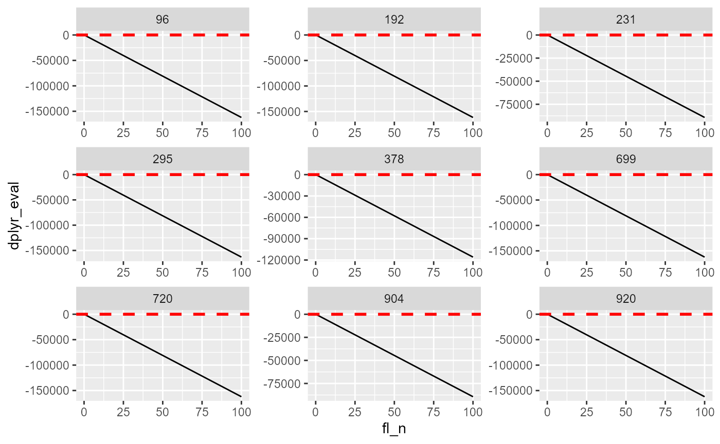
dplyr implementation of bisection
initialize matrix
first, initialize the matrix with \(a_0\) and \(b_0\), the initial min and max points:
# common prefix to make reshaping easier
st_bisec_prefix <- 'bisec_'
svr_a_lst <- paste0(st_bisec_prefix, 'a_0')
svr_b_lst <- paste0(st_bisec_prefix, 'b_0')
svr_fa_lst <- paste0(st_bisec_prefix, 'fa_0')
svr_fb_lst <- paste0(st_bisec_prefix, 'fb_0')

# add initial a and b
tb_states_choices_bisec <- tb_states_choices %>%
                            mutate(!!sym(svr_a_lst) := fl_n_min, !!sym(svr_b_lst) := fl_n_agg)

# evaluate function f(a_0) and f(b_0)
tb_states_choices_bisec <- tb_states_choices_bisec %>% rowwise() %>%
                            mutate(!!sym(svr_fa_lst) := ffi_nonlin_dplyrdo(fl_a, fl_alpha, !!sym(svr_a_lst),
                                                                          ar_nn_a, ar_nn_alpha,
                                                                          fl_n_agg, fl_rho),
                                   !!sym(svr_fb_lst) := ffi_nonlin_dplyrdo(fl_a, fl_alpha, !!sym(svr_b_lst),
                                                                          ar_nn_a, ar_nn_alpha,
                                                                          fl_n_agg, fl_rho))
# summarize
dim(tb_states_choices_bisec)
## [1] 1043 7
summary(tb_states_choices_bisec)## indi_id fl_a fl_alpha bisec_a_0 bisec_b_0
## Min. : 1.0 Min. :4.287 Min. :0.006687 Min. :0 Min. :100
## 1st Qu.: 261.5 1st Qu.:4.334 1st Qu.:0.006687 1st Qu.:0 1st Qu.:100
## Median : 522.0 Median :4.343 Median :0.012090 Median :0 Median :100
## Mean : 522.0 Mean :4.343 Mean :0.010321 Mean :0 Mean :100
## 3rd Qu.: 782.5 3rd Qu.:4.351 3rd Qu.:0.012090 3rd Qu.:0 3rd Qu.:100
## Max. :1043.0 Max. :4.417 Max. :0.013940 Max. :0 Max. :100
## bisec_fa_0 bisec_fb_0
## Min. :100 Min. :-163379
## 1st Qu.:100 1st Qu.:-161838
## Median :100 Median : -89227
## Mean :100 Mean :-114259
## 3rd Qu.:100 3rd Qu.: -88801
## Max. :100 Max. : -76145iterate and solve for f(p), update f(a) and f(b)
implement the dplyr based concurrent bisection algorithm.
# fl_tol = float tolerance criteria
# it_tol = number of interations to allow at most
fl_tol <- 10^-6
it_tol <- 100
# fl_p_dist2zr = distance to zero to initalize
fl_p_dist2zr <- 1000
it_cur <- 0
while (it_cur <= it_tol && fl_p_dist2zr >= fl_tol ) {

  it_cur <- it_cur + 1

  # new variables
  svr_a_cur <- paste0(st_bisec_prefix, 'a_', it_cur)
  svr_b_cur <- paste0(st_bisec_prefix, 'b_', it_cur)
  svr_fa_cur <- paste0(st_bisec_prefix, 'fa_', it_cur)
  svr_fb_cur <- paste0(st_bisec_prefix, 'fb_', it_cur)

  # evaluate function f(a_0) and f(b_0)
  # 1. generate p
  # 2. generate f_p
  # 3. generate f_p*f_a
  tb_states_choices_bisec <- tb_states_choices_bisec %>% rowwise() %>%
                              mutate(p = ((!!sym(svr_a_lst) + !!sym(svr_b_lst))/2)) %>%
                              mutate(f_p = ffi_nonlin_dplyrdo(fl_a, fl_alpha, p,
                                                              ar_nn_a, ar_nn_alpha,
                                                              fl_n_agg, fl_rho)) %>%
                              mutate(f_p_t_f_a = f_p*!!sym(svr_fa_lst))
  # fl_p_dist2zr = sum(abs(p))
  fl_p_dist2zr <- mean(abs(tb_states_choices_bisec %>% pull(f_p)))

  # update a and b
  tb_states_choices_bisec <- tb_states_choices_bisec %>%
                              mutate(!!sym(svr_a_cur) :=
                                       case_when(f_p_t_f_a < 0 ~ !!sym(svr_a_lst),
                                                 TRUE ~ p)) %>%
                              mutate(!!sym(svr_b_cur) :=
                                       case_when(f_p_t_f_a < 0 ~ p,
                                                 TRUE ~ !!sym(svr_b_lst)))
  # update f(a) and f(b)
  tb_states_choices_bisec <- tb_states_choices_bisec %>%
                              mutate(!!sym(svr_fa_cur) :=
                                       case_when(f_p_t_f_a < 0 ~ !!sym(svr_fa_lst),
                                                 TRUE ~ f_p)) %>%
                              mutate(!!sym(svr_fb_cur) :=
                                       case_when(f_p_t_f_a < 0 ~ f_p,
                                                 TRUE ~ !!sym(svr_fb_lst)))
  # save from last
  svr_a_lst <- svr_a_cur
  svr_b_lst <- svr_b_cur
  svr_fa_lst <- svr_fa_cur
  svr_fb_lst <- svr_fb_cur

  # summar current round
  print(paste0('it_cur:', it_cur, ', fl_p_dist2zr:', fl_p_dist2zr))
  summary(tb_states_choices_bisec %>% select(one_of(svr_a_cur, svr_b_cur, svr_fa_cur, svr_fb_cur)))
}
## [1] "it_cur:1, fl_p_dist2zr:57065.8515924507"
## [1] "it_cur:2, fl_p_dist2zr:28476.0859665553"
## [1] "it_cur:3, fl_p_dist2zr:14184.6282193769"
## [1] "it_cur:4, fl_p_dist2zr:7040.60930196585"
## [1] "it_cur:5, fl_p_dist2zr:3469.45353361675"
## [1] "it_cur:6, fl_p_dist2zr:1684.30185106396"
## [1] "it_cur:7, fl_p_dist2zr:791.938788974897"
## [1] "it_cur:8, fl_p_dist2zr:345.863486789484"
## [1] "it_cur:9, fl_p_dist2zr:122.878869797614"
## [1] "it_cur:10, fl_p_dist2zr:30.3977559686063"
## [1] "it_cur:11, fl_p_dist2zr:25.3181374761203"
## [1] "it_cur:12, fl_p_dist2zr:12.0886419051021"
## [1] "it_cur:13, fl_p_dist2zr:2.06815551406747"
## [1] "it_cur:14, fl_p_dist2zr:4.89604753960856"
## [1] "it_cur:15, fl_p_dist2zr:1.93331480031098"
## [1] "it_cur:16, fl_p_dist2zr:0.614579561133518"
## [1] "it_cur:17, fl_p_dist2zr:0.314081026590978"
## [1] "it_cur:18, fl_p_dist2zr:0.207595932727363"
## [1] "it_cur:19, fl_p_dist2zr:0.112869498156886"
## [1] "it_cur:20, fl_p_dist2zr:0.0559799114586833"
## [1] "it_cur:21, fl_p_dist2zr:0.027032944900061"
## [1] "it_cur:22, fl_p_dist2zr:0.0132672918026609"
## [1] "it_cur:23, fl_p_dist2zr:0.00680454432702988"
## [1] "it_cur:24, fl_p_dist2zr:0.00333360097714742"
## [1] "it_cur:25, fl_p_dist2zr:0.00168437455159884"
## [1] "it_cur:26, fl_p_dist2zr:0.000848467303071653"
## [1] "it_cur:27, fl_p_dist2zr:0.000427696340068737"
## [1] "it_cur:28, fl_p_dist2zr:0.000218673312373287"
## [1] "it_cur:29, fl_p_dist2zr:0.000108180725121156"
## [1] "it_cur:30, fl_p_dist2zr:5.24326238874592e-05"
## [1] "it_cur:31, fl_p_dist2zr:2.67010139017832e-05"
## [1] "it_cur:32, fl_p_dist2zr:1.33128324107031e-05"
## [1] "it_cur:33, fl_p_dist2zr:6.65284808581866e-06"
## [1] "it_cur:34, fl_p_dist2zr:3.34008954068542e-06"
## [1] "it_cur:35, fl_p_dist2zr:1.65812727955474e-06"
## [1] "it_cur:36, fl_p_dist2zr:8.52063209322296e-07"Reshape wide to long to wide
Table One–very wide
head(tb_states_choices_bisec, 10)## # A tibble: 10 x 154
## # Rowwise:
## indi_id fl_a fl_alpha bisec_a_0 bisec_b_0 bisec_fa_0 bisec_fb_0 p
## <int> <dbl> <dbl> <dbl> <dbl> <dbl> <dbl> <dbl>
## 1 1 4.34 0.00669 0 100 100 -161823. 0.0622
## 2 2 4.36 0.00925 0 100 100 -116164. 0.0862
## 3 3 4.35 0.00925 0 100 100 -116436. 0.0860
## 4 4 4.37 0.0139 0 100 100 -76535. 0.130
## 5 5 4.34 0.00669 0 100 100 -162038. 0.0621
## 6 6 4.36 0.0139 0 100 100 -76706. 0.130
## 7 7 4.34 0.00669 0 100 100 -162025. 0.0621
## 8 8 4.34 0.00669 0 100 100 -161980. 0.0621
## 9 9 4.36 0.0139 0 100 100 -76632. 0.130
## 10 10 4.33 0.0121 0 100 100 -89034. 0.112
## # ... with 146 more variables: f_p <dbl>, f_p_t_f_a <dbl>, bisec_a_1 <dbl>,
## # bisec_b_1 <dbl>, bisec_fa_1 <dbl>, bisec_fb_1 <dbl>, bisec_a_2 <dbl>,
## # bisec_b_2 <dbl>, bisec_fa_2 <dbl>, bisec_fb_2 <dbl>, bisec_a_3 <dbl>,
## # bisec_b_3 <dbl>, bisec_fa_3 <dbl>, bisec_fb_3 <dbl>, bisec_a_4 <dbl>,
## # bisec_b_4 <dbl>, bisec_fa_4 <dbl>, bisec_fb_4 <dbl>, bisec_a_5 <dbl>,
## # bisec_b_5 <dbl>, bisec_fa_5 <dbl>, bisec_fb_5 <dbl>, bisec_a_6 <dbl>,
## # bisec_b_6 <dbl>, bisec_fa_6 <dbl>, bisec_fb_6 <dbl>, bisec_a_7 <dbl>, ...## [1] "input allocated total sum: 100.000000033469"Table Two–very wide to very long
we want to treat the iteration count information that is the suffix of variable names as a variable by itself. additionally, we want to treat the a,b,fa,fb as a variable. structuring the data very long like this allows for easy graphing and other types of analysis. rather than dealing with many many variables, we have only 3 core variables that store bisection iteration information.
here we use the very nice pivot_longer function. note that to achieve this, we put a common prefix in front of the variables we wanted to convert to long. this is helpful, because we can easily identify which variables need to be reshaped.
# new variables
svr_bisect_iter <- 'biseciter'
svr_abfafb_long_name <- 'varname'
svr_number_col <- 'value'
svr_id_bisect_iter <- paste0(svr_id_var, '_bisect_ier')

# pivot wide to very long
set.seed(123)
tb_states_choices_bisec_long <-
  tb_states_choices_bisec[sample(dim(tb_states_choices_bisec)[1], 9, replace=FALSE),] %>%
  pivot_longer(
    cols = starts_with(st_bisec_prefix),
    names_to = c(svr_abfafb_long_name, svr_bisect_iter),
    names_pattern = paste0(st_bisec_prefix, "(.*)_(.*)"),
    values_to = svr_number_col
  )

# print
summary(tb_states_choices_bisec_long)
## indi_id fl_a fl_alpha p
## Min. :179.0 Min. :4.330 Min. :0.006687 Min. :0.06205
## 1st Qu.:415.0 1st Qu.:4.333 1st Qu.:0.009251 1st Qu.:0.08607
## Median :526.0 Median :4.350 Median :0.012090 Median :0.11231
## Mean :521.3 Mean :4.346 Mean :0.011396 Mean :0.10591
## 3rd Qu.:665.0 3rd Qu.:4.356 3rd Qu.:0.013940 3rd Qu.:0.12969
## Max. :938.0 Max. :4.361 Max. :0.013940 Max. :0.12983
## f_p f_p_t_f_a varname
## Min. :-1.383e-06 Min. :-1.334e-12 Length:1332
## 1st Qu.:-8.178e-07 1st Qu.:-4.099e-13 Class :character
## Median :-1.467e-07 Median :-1.525e-13 Mode :character
## Mean :-3.205e-07 Mean : 1.368e-13
## 3rd Qu.: 1.672e-07 3rd Qu.: 2.153e-13
## Max. : 1.022e-06 Max. : 3.444e-12
## biseciter value
## Length:1332 Min. :-162130.75
## Class :character 1st Qu.: 0.00
## Mode :character Median : 0.06
## Mean : -1374.64
## 3rd Qu.: 0.13
## Max. : 100.00## # A tibble: 30 x 6
## indi_id fl_a fl_alpha varname biseciter value
## <int> <dbl> <dbl> <chr> <chr> <dbl>
## 1 415 4.33 0.00669 a 0 0
## 2 415 4.33 0.00669 b 0 100
## 3 415 4.33 0.00669 fa 0 100
## 4 415 4.33 0.00669 fb 0 -162131.
## 5 415 4.33 0.00669 a 1 0
## 6 415 4.33 0.00669 b 1 50
## 7 415 4.33 0.00669 fa 1 100
## 8 415 4.33 0.00669 fb 1 -80965.
## 9 415 4.33 0.00669 a 2 0
## 10 415 4.33 0.00669 b 2 25
## # ... with 20 more rows## # A tibble: 30 x 6
## indi_id fl_a fl_alpha varname biseciter value
## <int> <dbl> <dbl> <chr> <chr> <dbl>
## 1 709 4.33 0.0121 fa 29 0.0000610
## 2 709 4.33 0.0121 fb 29 -0.000105
## 3 709 4.33 0.0121 a 30 0.112
## 4 709 4.33 0.0121 b 30 0.112
## 5 709 4.33 0.0121 fa 30 0.0000610
## 6 709 4.33 0.0121 fb 30 -0.0000222
## 7 709 4.33 0.0121 a 31 0.112
## 8 709 4.33 0.0121 b 31 0.112
## 9 709 4.33 0.0121 fa 31 0.0000194
## 10 709 4.33 0.0121 fb 31 -0.0000222
## # ... with 20 more rowsTable Two–very very long to wider again
but the previous results are too long, with the a, b, fa, and fb all in one column as different categories, they are really not different categories, they are in fact different types of variables. so we want to spread those four categories of this variable into four columns, each one representing the a, b, fa, and fb values. the rows would then be uniquly identified by the iteration counter and individual id.
# pivot wide to very long to a little wide
tb_states_choices_bisec_wider <- tb_states_choices_bisec_long %>%
  pivot_wider(
    names_from = !!sym(svr_abfafb_long_name),
    values_from = svr_number_col
  )
## Note: Using an external vector in selections is ambiguous.
## i Use `all_of(svr_number_col)` instead of `svr_number_col` to silence this message.
## i See <https://tidyselect.r-lib.org/reference/faq-external-vector.html>.
## This message is displayed once per session.
# print
summary(tb_states_choices_bisec_wider)
## indi_id fl_a fl_alpha p
## Min. :179.0 Min. :4.330 Min. :0.006687 Min. :0.06205
## 1st Qu.:415.0 1st Qu.:4.333 1st Qu.:0.009251 1st Qu.:0.08607
## Median :526.0 Median :4.350 Median :0.012090 Median :0.11231
## Mean :521.3 Mean :4.346 Mean :0.011396 Mean :0.10591
## 3rd Qu.:665.0 3rd Qu.:4.356 3rd Qu.:0.013940 3rd Qu.:0.12969
## Max. :938.0 Max. :4.361 Max. :0.013940 Max. :0.12983
## f_p f_p_t_f_a biseciter a
## Min. :-1.383e-06 Min. :-1.334e-12 Length:333 Min. :0.00000
## 1st Qu.:-8.178e-07 1st Qu.:-4.099e-13 Class :character 1st Qu.:0.00000
## Median :-1.467e-07 Median :-1.525e-13 Mode :character Median :0.08607
## Mean :-3.205e-07 Mean : 1.368e-13 Mean :0.07498
## 3rd Qu.: 1.672e-07 3rd Qu.: 2.153e-13 3rd Qu.:0.12817
## Max. : 1.022e-06 Max. : 3.444e-12 Max. :0.12983
## b fa fb
## Min. : 0.06205 Min. : 0.00000 Min. :-162130.75
## 1st Qu.: 0.11195 1st Qu.: 0.00033 1st Qu.: -126.98
## Median : 0.12969 Median : 0.15876 Median : -0.09
## Mean : 5.48039 Mean : 29.47787 Mean : -5533.61
## 3rd Qu.: 0.19531 3rd Qu.:100.00000 3rd Qu.: 0.00
## Max. :100.00000 Max. :100.00000 Max. : 0.00## # A tibble: 30 x 8
## indi_id fl_a fl_alpha biseciter a b fa fb
## <int> <dbl> <dbl> <chr> <dbl> <dbl> <dbl> <dbl>
## 1 415 4.33 0.00669 0 0 100 100 -162131.
## 2 415 4.33 0.00669 1 0 50 100 -80965.
## 3 415 4.33 0.00669 2 0 25 100 -40407.
## 4 415 4.33 0.00669 3 0 12.5 100 -20141.
## 5 415 4.33 0.00669 4 0 6.25 100 -10014.
## 6 415 4.33 0.00669 5 0 3.12 100 -4954.
## 7 415 4.33 0.00669 6 0 1.56 100 -2425.
## 8 415 4.33 0.00669 7 0 0.781 100 -1162.
## 9 415 4.33 0.00669 8 0 0.391 100 -531.
## 10 415 4.33 0.00669 9 0 0.195 100 -215.
## # ... with 20 more rows## # A tibble: 30 x 8
## indi_id fl_a fl_alpha biseciter a b fa fb
## <int> <dbl> <dbl> <chr> <dbl> <dbl> <dbl> <dbl>
## 1 709 4.33 0.0121 7 0 0.781 100 -598.
## 2 709 4.33 0.0121 8 0 0.391 100 -249.
## 3 709 4.33 0.0121 9 0 0.195 100 -74.4
## 4 709 4.33 0.0121 10 0.0977 0.195 12.8 -74.4
## 5 709 4.33 0.0121 11 0.0977 0.146 12.8 -30.8
## 6 709 4.33 0.0121 12 0.0977 0.122 12.8 -9.04
## 7 709 4.33 0.0121 13 0.110 0.122 1.86 -9.04
## 8 709 4.33 0.0121 14 0.110 0.116 1.86 -3.59
## 9 709 4.33 0.0121 15 0.110 0.113 1.86 -0.863
## 10 709 4.33 0.0121 16 0.111 0.113 0.499 -0.863
## # ... with 20 more rowsGraph Bisection Iteration results
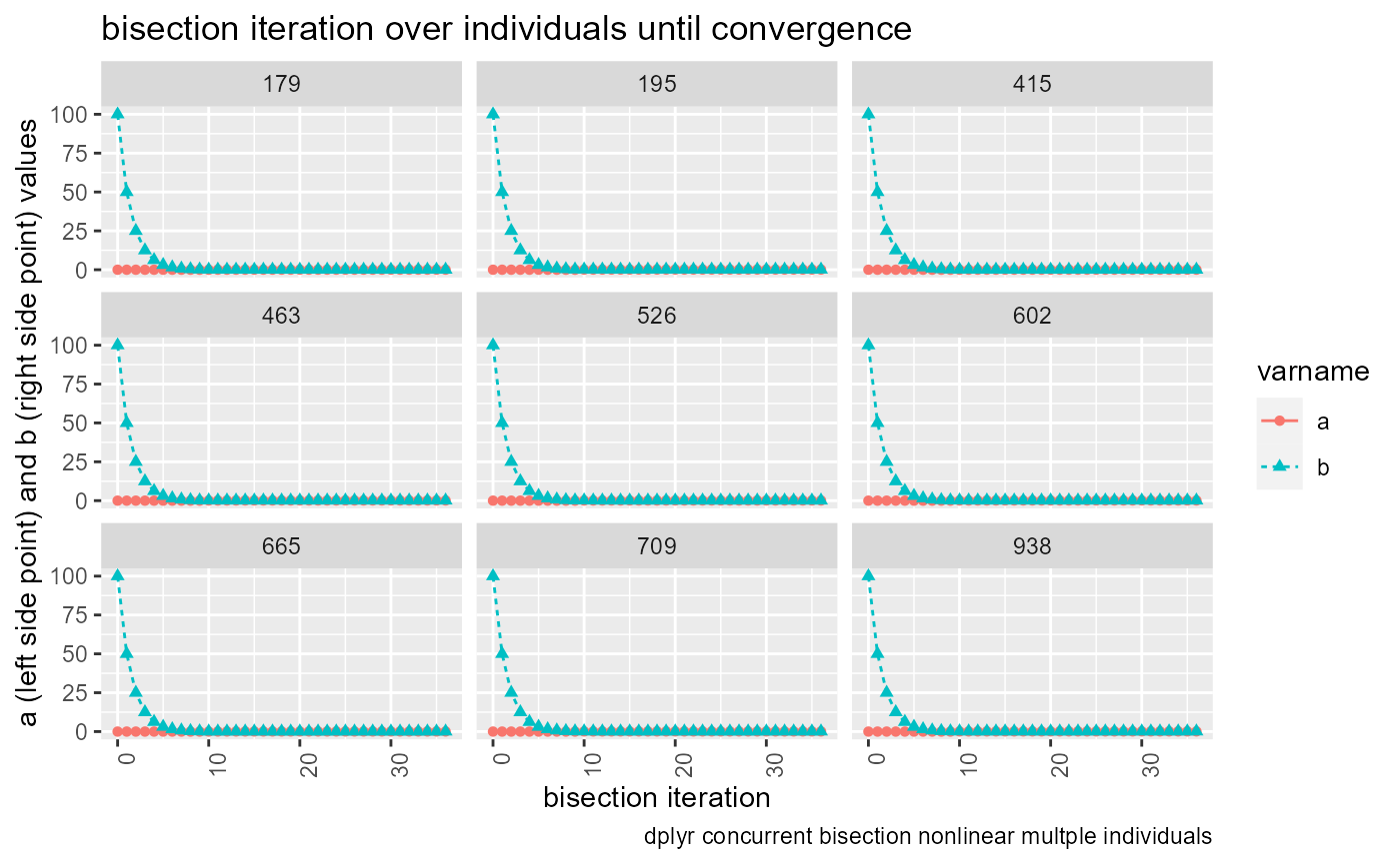
actually we want to graph based on the long results, not the wider. wider easier to view in table.
# graph results
lineplot <- tb_states_choices_bisec_long %>%
    mutate(!!sym(svr_bisect_iter) := as.numeric(!!sym(svr_bisect_iter))) %>%
    filter(!!sym(svr_abfafb_long_name) %in% c('a', 'b')) %>%
    ggplot(aes(x=!!sym(svr_bisect_iter), y=!!sym(svr_number_col),
               colour=!!sym(svr_abfafb_long_name),
               linetype=!!sym(svr_abfafb_long_name),
               shape=!!sym(svr_abfafb_long_name))) +
        facet_wrap( ~ indi_id) +
        geom_line() +
        geom_point() +
        labs(title = 'bisection iteration over individuals until convergence',
             x = 'bisection iteration',
             y = 'a (left side point) and b (right side point) values',
             caption = 'dplyr concurrent bisection nonlinear multple individuals') +
      theme(axis.text.x = element_text(angle = 90, hjust = 1))
print(lineplot)