Solve Roots for N (Rows) Strictly Monotonic Functions
Source:vignettes/fv_opti_bisect_pmap_multi.Rmd
fv_opti_bisect_pmap_multi.RmdSolve for roots for the same function across N sets of parameter values. This file works out how the ff_opti_bisect_pmap_multi function works from Fan’s REconTools Package. Also see a closely related file from R4Econ, DPLYR Bisection, which works out in greater detail the bisection algorithm.
We want solve for function \(0=f(z_{ij}, x_i, y_i, \textbf{X}, \textbf{Y}, c, d)\). There are \(i\) functions that have \(i\) specific \(x\) and \(y\). For each \(i\) function, we evaluate along a grid of feasible values for \(z\), over \(j\in J\) grid points, potentially looking for the \(j\) that is closest to the root. \(j\) could be interpreted as iterations. \(\textbf{X}\) and \(\textbf{Y}\) are arrays common across the \(i\) equations, and \(c\) and \(d\) are constants.
As we iterate over \(j\), find the \(z_{ij}\) that is \(i\) specific that allows for \(f_{i}(z_{ij})=0\).
In the code below, we develop the bisection code line by line, then we write it as a function using pmap. At the end, we test the concurrent bisection code over tibble dataframe with a set of straight lines (negative intercepts and positive slopes), and the log-linear solution for optimal allocation function from fan’s PrjOptiAlloc Project.
Bisection Algorithm
This is how I implement the bisection algorithm, when we know the bounding minimum and maximum to be below and above zero already.
- Evaluate \(f^0_a = f(a^0)\) and \(f^0_b = f(b^0)\), min and max points.
- Evaluate at \(f^0_p = f(p^0)\), where \(p_0 = \frac{a^0+b^0}{2}\).
- if \(f^i_a \cdot f^i_p < 0\), then \(b_{i+1} = p_i\), else, \(a_{i+1} = p_i\) and \(f^{i+1}_a = p_i\).
- iteratre until convergence.
And for the function we want to bisect over, as stated earlier, it has three types of variables:
- variables in file for grouping, each group is an individual for whom we want to calculate optimal choice for using bisection.
- variables that change each row and each iteration, the root we are looking for.
- scalar and array values that are applied to every row and persist across iterations.
Set up for Implementation
Invoking the algorithm uses several key tidyverse functions:
- pmap from purrr to evaluate function row by row.
- case_when from dplyr to set new lower and upper bound.
- pivot_wider and pivot_longer from tidyr to reshape resulting file if record all iteration results.
Set up Input Arrays
There is a function that takes \(M=Q+P\) inputs, we want to evaluate this function \(N\) times. Each time, there are \(M\) inputs, where all but \(Q\) of the \(M\) inputs, meaning \(P\) of the \(M\) inputs, are the same. In particular, \(P=Q*N\).
\[M = Q+P = Q + Q*N\]
Now we need to expand this by the number of choice grid. Each row, representing one equation, is expanded by the number of choice grids. We are graphically searching, or rather brute force searching, which means if we have 100 individuals, we want to plot out the nonlinear equation for each of these lines, and show graphically where each line crosses zero. We achieve this, by evaluating the equation for each of the 100 individuals along a grid of feasible choices.
In this problem here, the feasible choices are shared across individuals.
# Parameters
fl_rho = 0.20
svr_id_var = 'INDI_ID'

# it_child_count = N, the number of children
it_N_child_cnt = 9
# it_heter_param = Q, number of parameters that are heterogeneous across children
it_Q_hetpa_cnt = 2

# P fixed parameters, nN is N dimensional, nP is P dimensional
ar_nN_A = seq(-2, 2, length.out = it_N_child_cnt)
ar_nN_alpha = seq(0.1, 0.9, length.out = it_N_child_cnt)
ar_nP_A_alpha = c(ar_nN_A, ar_nN_alpha)

# N by Q varying parameters
mt_nN_by_nQ_A_alpha = cbind(ar_nN_A, ar_nN_alpha)

# Choice Grid for nutritional feasible choices for each
fl_N_agg = 100
fl_N_min = 0

# Mesh Expand
tb_states_choices <- as_tibble(mt_nN_by_nQ_A_alpha) %>% rowid_to_column(var=svr_id_var)
ar_st_col_names = c(svr_id_var,'fl_A', 'fl_alpha')
tb_states_choices <- tb_states_choices %>% rename_all(~c(ar_st_col_names))

# display
summary(tb_states_choices)
#>     INDI_ID       fl_A       fl_alpha
#>  Min.   :1   Min.   :-2   Min.   :0.1
#>  1st Qu.:3   1st Qu.:-1   1st Qu.:0.3
#>  Median :5   Median : 0   Median :0.5
#>  Mean   :5   Mean   : 0   Mean   :0.5
#>  3rd Qu.:7   3rd Qu.: 1   3rd Qu.:0.7
#>  Max.   :9   Max.   : 2   Max.   :0.9
kable(tb_states_choices) %>%
kable_styling(bootstrap_options = c("striped", "hover", "condensed", "responsive"))| INDI_ID | fl_A | fl_alpha |
|---|---|---|
| 1 | -2.0 | 0.1 |
| 2 | -1.5 | 0.2 |
| 3 | -1.0 | 0.3 |
| 4 | -0.5 | 0.4 |
| 5 | 0.0 | 0.5 |
| 6 | 0.5 | 0.6 |
| 7 | 1.0 | 0.7 |
| 8 | 1.5 | 0.8 |
| 9 | 2.0 | 0.9 |
Create Nonlinear Root Function
These is a test functions over which we will searh for roots.
# Define Implicit Function
ffi_nonlin_dplyrdo <- function(fl_A, fl_alpha, fl_N, ar_A, ar_alpha, fl_N_agg, fl_rho){
  # scalar value that are row-specific, in dataframe already: *fl_A*, *fl_alpha*, *fl_N*
  # array and scalars not in dataframe, common all rows: *ar_A*, *ar_alpha*, *fl_N_agg*, *fl_rho*

  # Test Parameters
  # ar_A = ar_nN_A
  # ar_alpha = ar_nN_alpha
  # fl_N = 100
  # fl_rho = -1
  # fl_N_q = 10

  # Apply Function
  ar_p1_s1 = exp((fl_A - ar_A)*fl_rho)
  ar_p1_s2 = (fl_alpha/ar_alpha)
  ar_p1_s3 = (1/(ar_alpha*fl_rho - 1))
  ar_p1 = (ar_p1_s1*ar_p1_s2)^ar_p1_s3
  ar_p2 = fl_N^((fl_alpha*fl_rho-1)/(ar_alpha*fl_rho-1))
  ar_overall = ar_p1*ar_p2
  fl_overall = fl_N_agg - sum(ar_overall)

  return(fl_overall)
}
Step by Step Implmentation of Algorithm
Generate New columns of a and b as we iteratre, do not need to store p, p is temporary. Evaluate the function below which we have already tested, but now, in the dataframe before generating all permutations, tb_states_choices, now the fl_N element will be changing with each iteration, it will be row specific. fl_N are first min and max, then each subsequent ps.
Initialize Matrix
First, initialize the matrix with \(a_0\) and \(b_0\), the initial min and max points:
# common prefix to make reshaping easier
st_bisec_prefix <- 'bisec_'
svr_a_lst <- paste0(st_bisec_prefix, 'a_0')
svr_b_lst <- paste0(st_bisec_prefix, 'b_0')
svr_fa_lst <- paste0(st_bisec_prefix, 'fa_0')
svr_fb_lst <- paste0(st_bisec_prefix, 'fb_0')

# Add initial a and b
tb_states_choices_bisec <- tb_states_choices %>%
                            mutate(!!sym(svr_a_lst) := fl_N_min, !!sym(svr_b_lst) := fl_N_agg)

# Evaluate function f(a_0) and f(b_0)
tb_states_choices_bisec <- tb_states_choices_bisec %>% rowwise() %>%
                            mutate(!!sym(svr_fa_lst) := ffi_nonlin_dplyrdo(fl_A, fl_alpha, !!sym(svr_a_lst),
                                                                          ar_nN_A, ar_nN_alpha,
                                                                          fl_N_agg, fl_rho),
                                   !!sym(svr_fb_lst) := ffi_nonlin_dplyrdo(fl_A, fl_alpha, !!sym(svr_b_lst),
                                                                          ar_nN_A, ar_nN_alpha,
                                                                          fl_N_agg, fl_rho))
# Summarize
dim(tb_states_choices_bisec)
#> [1] 9 7
summary(tb_states_choices_bisec)
#>     INDI_ID       fl_A       fl_alpha     bisec_a_0   bisec_b_0     bisec_fa_0
#>  Min.   :1   Min.   :-2   Min.   :0.1   Min.   :0   Min.   :100   Min.   :100
#>  1st Qu.:3   1st Qu.:-1   1st Qu.:0.3   1st Qu.:0   1st Qu.:100   1st Qu.:100
#>  Median :5   Median : 0   Median :0.5   Median :0   Median :100   Median :100
#>  Mean   :5   Mean   : 0   Mean   :0.5   Mean   :0   Mean   :100   Mean   :100
#>  3rd Qu.:7   3rd Qu.: 1   3rd Qu.:0.7   3rd Qu.:0   3rd Qu.:100   3rd Qu.:100
#>  Max.   :9   Max.   : 2   Max.   :0.9   Max.   :0   Max.   :100   Max.   :100
#>    bisec_fb_0
#>  Min.   :-24328.4
#>  1st Qu.: -4157.8
#>  Median : -1386.7
#>  Mean   : -4737.0
#>  3rd Qu.:  -538.0
#>  Max.   :  -202.9
Iterate and Solve for f(p), update f(a) and f(b)
Implement the DPLYR based Concurrent bisection algorithm.
# fl_tol = float tolerance criteria
# it_tol = number of interations to allow at most
fl_tol <- 10^-2
it_tol <- 100

# fl_p_dist2zr = distance to zero to initalize
fl_p_dist2zr <- 1000
it_cur <- 0
while (it_cur <= it_tol && fl_p_dist2zr >= fl_tol ) {

  it_cur <- it_cur + 1

  # New Variables
  svr_a_cur <- paste0(st_bisec_prefix, 'a_', it_cur)
  svr_b_cur <- paste0(st_bisec_prefix, 'b_', it_cur)
  svr_fa_cur <- paste0(st_bisec_prefix, 'fa_', it_cur)
  svr_fb_cur <- paste0(st_bisec_prefix, 'fb_', it_cur)

  # Evaluate function f(a_0) and f(b_0)
  # 1. generate p
  # 2. generate f_p
  # 3. generate f_p*f_a
  tb_states_choices_bisec <- tb_states_choices_bisec %>% rowwise() %>%
                              mutate(p = ((!!sym(svr_a_lst) + !!sym(svr_b_lst))/2)) %>%
                              mutate(f_p = ffi_nonlin_dplyrdo(fl_A, fl_alpha, p,
                                                              ar_nN_A, ar_nN_alpha,
                                                              fl_N_agg, fl_rho)) %>%
                              mutate(f_p_t_f_a = f_p*!!sym(svr_fa_lst))
  # fl_p_dist2zr = sum(abs(p))
  fl_p_dist2zr <- mean(abs(tb_states_choices_bisec %>% pull(f_p)))

  # Update a and b
  tb_states_choices_bisec <- tb_states_choices_bisec %>%
                              mutate(!!sym(svr_a_cur) :=
                                       case_when(f_p_t_f_a < 0 ~ !!sym(svr_a_lst),
                                                 TRUE ~ p)) %>%
                              mutate(!!sym(svr_b_cur) :=
                                       case_when(f_p_t_f_a < 0 ~ p,
                                                 TRUE ~ !!sym(svr_b_lst)))
  # Update f(a) and f(b)
  tb_states_choices_bisec <- tb_states_choices_bisec %>%
                              mutate(!!sym(svr_fa_cur) :=
                                       case_when(f_p_t_f_a < 0 ~ !!sym(svr_fa_lst),
                                                 TRUE ~ f_p)) %>%
                              mutate(!!sym(svr_fb_cur) :=
                                       case_when(f_p_t_f_a < 0 ~ f_p,
                                                 TRUE ~ !!sym(svr_fb_lst)))
  # Save from last
  svr_a_lst <- svr_a_cur
  svr_b_lst <- svr_b_cur
  svr_fa_lst <- svr_fa_cur
  svr_fb_lst <- svr_fb_cur

  # Summar current round
  print(paste0('it_cur:', it_cur, ', fl_p_dist2zr:', fl_p_dist2zr))
  summary(tb_states_choices_bisec %>% select(one_of(svr_a_cur, svr_b_cur, svr_fa_cur, svr_fb_cur)))
}
#> [1] "it_cur:1, fl_p_dist2zr:2110.89580734824"
#> [1] "it_cur:2, fl_p_dist2zr:916.745756204857"
#> [1] "it_cur:3, fl_p_dist2zr:387.351245210125"
#> [1] "it_cur:4, fl_p_dist2zr:155.209641366984"
#> [1] "it_cur:5, fl_p_dist2zr:58.1570911334532"
#> [1] "it_cur:6, fl_p_dist2zr:22.2118416173139"
#> [1] "it_cur:7, fl_p_dist2zr:8.74989971240847"
#> [1] "it_cur:8, fl_p_dist2zr:7.15872428611325"
#> [1] "it_cur:9, fl_p_dist2zr:3.58472422897695"
#> [1] "it_cur:10, fl_p_dist2zr:1.50543493747611"
#> [1] "it_cur:11, fl_p_dist2zr:0.527052368572328"
#> [1] "it_cur:12, fl_p_dist2zr:0.360171292121815"
#> [1] "it_cur:13, fl_p_dist2zr:0.0545239655746409"
#> [1] "it_cur:14, fl_p_dist2zr:0.152964071033218"
#> [1] "it_cur:15, fl_p_dist2zr:0.0593547942434943"
#> [1] "it_cur:16, fl_p_dist2zr:0.030716694397913"
#> [1] "it_cur:17, fl_p_dist2zr:0.0177772298500779"
#> [1] "it_cur:18, fl_p_dist2zr:0.00644396015251105"
Reshape Wide to long to Wide
To view results easily, how iterations improved to help us find the roots, convert table from wide to long. Pivot twice. This allows us to easily graph out how bisection is working out iterationby iteration.
Here, we will first show what the raw table looks like, the wide only table, and then show the long version, and finally the version that is medium wide.
# New variables
svr_bisect_iter <- 'biseciter'
svr_abfafb_long_name <- 'varname'
svr_number_col <- 'value'
svr_id_bisect_iter <- paste0(svr_id_var, '_bisect_ier')

# Pivot wide to very long
tb_states_choices_bisec_long <- tb_states_choices_bisec %>%
  pivot_longer(
    cols = starts_with(st_bisec_prefix),
    names_to = c(svr_abfafb_long_name, svr_bisect_iter),
    names_pattern = paste0(st_bisec_prefix, "(.*)_(.*)"),
    values_to = svr_number_col
  )

# Print
summary(tb_states_choices_bisec_long)
#>     INDI_ID       fl_A       fl_alpha         p                f_p
#>  Min.   :1   Min.   :-2   Min.   :0.1   Min.   : 0.8427   Min.   :-1.874e-02
#>  1st Qu.:3   1st Qu.:-1   1st Qu.:0.3   1st Qu.: 3.3298   1st Qu.:-2.887e-03
#>  Median :5   Median : 0   Median :0.5   Median : 7.7381   Median : 1.987e-05
#>  Mean   :5   Mean   : 0   Mean   :0.5   Mean   :11.1111   Mean   :-2.921e-04
#>  3rd Qu.:7   3rd Qu.: 1   3rd Qu.:0.7   3rd Qu.:15.8810   3rd Qu.: 2.626e-03
#>  Max.   :9   Max.   : 2   Max.   :0.9   Max.   :31.5121   Max.   : 2.000e-02
#>    f_p_t_f_a            varname           biseciter
#>  Min.   :-6.210e-04   Length:684         Length:684
#>  1st Qu.:-6.641e-06   Class :character   Class :character
#>  Median : 2.350e-08   Mode  :character   Mode  :character
#>  Mean   : 2.613e-05
#>  3rd Qu.: 2.393e-05
#>  Max.   : 8.464e-04
#>      value
#>  Min.   :-24328.416
#>  1st Qu.:     0.000
#>  Median :     1.917
#>  Mean   :   -97.563
#>  3rd Qu.:    15.674
#>  Max.   :   100.000
head(tb_states_choices_bisec_long %>% select(-one_of('p','f_p','f_p_t_f_a')), 30)
#> # A tibble: 30 x 6
#>    INDI_ID  fl_A fl_alpha varname biseciter   value
#>      <int> <dbl>    <dbl> <chr>   <chr>       <dbl>
#>  1       1    -2      0.1 a       0              0
#>  2       1    -2      0.1 b       0            100
#>  3       1    -2      0.1 fa      0            100
#>  4       1    -2      0.1 fb      0         -24328.
#>  5       1    -2      0.1 a       1              0
#>  6       1    -2      0.1 b       1             50
#>  7       1    -2      0.1 fa      1            100
#>  8       1    -2      0.1 fb      1         -10867.
#>  9       1    -2      0.1 a       2              0
#> 10       1    -2      0.1 b       2             25
#> # ... with 20 more rows
tail(tb_states_choices_bisec_long %>% select(-one_of('p','f_p','f_p_t_f_a')), 30)
#> # A tibble: 30 x 6
#>    INDI_ID  fl_A fl_alpha varname biseciter   value
#>      <int> <dbl>    <dbl> <chr>   <chr>       <dbl>
#>  1       9     2      0.9 fa      11         0.0546
#>  2       9     2      0.9 fb      11        -0.0940
#>  3       9     2      0.9 a       12        31.5
#>  4       9     2      0.9 b       12        31.5
#>  5       9     2      0.9 fa      12         0.0546
#>  6       9     2      0.9 fb      12        -0.0197
#>  7       9     2      0.9 a       13        31.5
#>  8       9     2      0.9 b       13        31.5
#>  9       9     2      0.9 fa      13         0.0174
#> 10       9     2      0.9 fb      13        -0.0197
#> # ... with 20 more rows

# Pivot wide to very long to a little wide
tb_states_choices_bisec_wider <- tb_states_choices_bisec_long %>%
  pivot_wider(
    names_from = !!sym(svr_abfafb_long_name),
    values_from = svr_number_col
  )
#> Note: Using an external vector in selections is ambiguous.
#> i Use `all_of(svr_number_col)` instead of `svr_number_col` to silence this message.
#> i See <https://tidyselect.r-lib.org/reference/faq-external-vector.html>.
#> This message is displayed once per session.

# Print
summary(tb_states_choices_bisec_wider)
#>     INDI_ID       fl_A       fl_alpha         p                f_p
#>  Min.   :1   Min.   :-2   Min.   :0.1   Min.   : 0.8427   Min.   :-1.874e-02
#>  1st Qu.:3   1st Qu.:-1   1st Qu.:0.3   1st Qu.: 3.3298   1st Qu.:-2.887e-03
#>  Median :5   Median : 0   Median :0.5   Median : 7.7381   Median : 1.987e-05
#>  Mean   :5   Mean   : 0   Mean   :0.5   Mean   :11.1111   Mean   :-2.921e-04
#>  3rd Qu.:7   3rd Qu.: 1   3rd Qu.:0.7   3rd Qu.:15.8810   3rd Qu.: 2.626e-03
#>  Max.   :9   Max.   : 2   Max.   :0.9   Max.   :31.5121   Max.   : 2.000e-02
#>    f_p_t_f_a           biseciter               a                 b
#>  Min.   :-6.210e-04   Length:171         Min.   : 0.0000   Min.   :  0.8427
#>  1st Qu.:-6.641e-06   Class :character   1st Qu.: 0.8057   1st Qu.:  5.2093
#>  Median : 2.350e-08   Mode  :character   Median : 5.2002   Median : 11.7188
#>  Mean   : 2.613e-05                      Mean   : 8.9430   Mean   : 19.4693
#>  3rd Qu.: 2.393e-05                      3rd Qu.:15.6250   3rd Qu.: 25.0000
#>  Max.   : 8.464e-04                      Max.   :31.5121   Max.   :100.0000
#>        fa                  fb
#>  Min.   :  0.00002   Min.   :-24328.416
#>  1st Qu.:  0.04899   1st Qu.:   -45.805
#>  Median :  0.79745   Median :    -1.329
#>  Mean   : 25.85998   Mean   :  -444.523
#>  3rd Qu.: 21.38681   3rd Qu.:    -0.064
#>  Max.   :100.00000   Max.   :     0.000
head(tb_states_choices_bisec_wider %>% select(-one_of('p','f_p','f_p_t_f_a')), 30)
#> # A tibble: 30 x 8
#>    INDI_ID  fl_A fl_alpha biseciter     a       b     fa       fb
#>      <int> <dbl>    <dbl> <chr>     <dbl>   <dbl>  <dbl>    <dbl>
#>  1       1    -2      0.1 0         0     100     100    -24328.
#>  2       1    -2      0.1 1         0      50     100    -10867.
#>  3       1    -2      0.1 2         0      25     100     -4828.
#>  4       1    -2      0.1 3         0      12.5   100     -2117.
#>  5       1    -2      0.1 4         0       6.25  100      -898.
#>  6       1    -2      0.1 5         0       3.12  100      -350.
#>  7       1    -2      0.1 6         0       1.56  100      -103.
#>  8       1    -2      0.1 7         0.781   1.56    8.29   -103.
#>  9       1    -2      0.1 8         0.781   1.17    8.29    -46.0
#> 10       1    -2      0.1 9         0.781   0.977   8.29    -18.4
#> # ... with 20 more rows
tail(tb_states_choices_bisec_wider %>% select(-one_of('p','f_p','f_p_t_f_a')), 30)
#> # A tibble: 30 x 8
#>    INDI_ID  fl_A fl_alpha biseciter     a     b      fa         fb
#>      <int> <dbl>    <dbl> <chr>     <dbl> <dbl>   <dbl>      <dbl>
#>  1       8   1.5      0.8 8          22.3  22.7 0.579   -1.13
#>  2       8   1.5      0.8 9          22.3  22.5 0.579   -0.278
#>  3       8   1.5      0.8 10         22.4  22.5 0.150   -0.278
#>  4       8   1.5      0.8 11         22.4  22.4 0.150   -0.0636
#>  5       8   1.5      0.8 12         22.4  22.4 0.0434  -0.0636
#>  6       8   1.5      0.8 13         22.4  22.4 0.0434  -0.0101
#>  7       8   1.5      0.8 14         22.4  22.4 0.0167  -0.0101
#>  8       8   1.5      0.8 15         22.4  22.4 0.00327 -0.0101
#>  9       8   1.5      0.8 16         22.4  22.4 0.00327 -0.00342
#> 10       8   1.5      0.8 17         22.4  22.4 0.00327 -0.0000761
#> # ... with 20 more rows
Graph Bisection Iteration Results
Actually we want to graph based on the long results, not the wider. Wider easier to view in table.
# Graph results
lineplot <- tb_states_choices_bisec_long %>%
    mutate(!!sym(svr_bisect_iter) := as.numeric(!!sym(svr_bisect_iter))) %>%
    filter(!!sym(svr_abfafb_long_name) %in% c('a', 'b')) %>%
    ggplot(aes(x=!!sym(svr_bisect_iter), y=!!sym(svr_number_col),
               colour=!!sym(svr_abfafb_long_name),
               linetype=!!sym(svr_abfafb_long_name),
               shape=!!sym(svr_abfafb_long_name))) +
        facet_wrap( ~ INDI_ID) +
        geom_line() +
        geom_point() +
        labs(title = 'Bisection Iteration over individuals Until Convergence',
             x = 'Bisection Iteration',
             y = 'a (left side point) and b (right side point) values',
             caption = 'DPLYR concurrent bisection nonlinear multple individuals') +
      theme(axis.text.x = element_text(angle = 90, hjust = 1))
print(lineplot)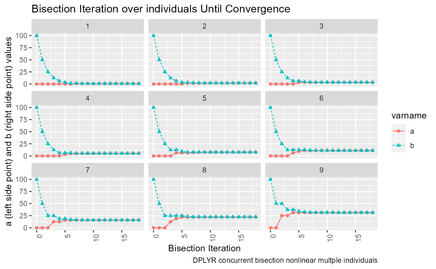
Implement Bisection as A Function over Dataframe
Define Bisection Algorithm Function
Note the df input must have the not hard-coded input variables in fc_withroot, identical names. In particular, svr_bisect_solu should specify the name of the root variable: the x variable, which we are changing to solve for zero, whatever it is called in the df dataframe.
Inputs:
- ls_svr_df_in_func: string list of variables in df that are inputs for fc_withroot.
- svr_root_x: the x variable name that appears n fc_withroot.
fv_opti_bisect_pmap_multi_test <- function(df, fc_withroot,
                                           fl_lower_x, fl_upper_x,
                                           ls_svr_df_in_func,
                                           svr_root_x = 'x',
                                           it_iter_tol = 50, fl_zero_tol = 10^-5,
                                           bl_keep_iter = TRUE,
                                           st_bisec_prefix = 'bisec_',
                                           st_lower_x = 'a', st_lower_fx = 'fa',
                                           st_upper_x = 'b', st_upper_fx = 'fb') {


# A. common prefix to make reshaping easier
svr_a_lst <- paste0(st_bisec_prefix, st_lower_x, '_0')
svr_b_lst <- paste0(st_bisec_prefix, st_upper_x, '_0')
svr_fa_lst <- paste0(st_bisec_prefix, st_lower_fx, '_0')
svr_fb_lst <- paste0(st_bisec_prefix, st_upper_fx, '_0')
svr_fxvr_name <- paste0('f', svr_root_x)
ls_pmap_vars <- unique(c(ls_svr_df_in_func, svr_root_x))

# B. Add initial a and b
df_bisec <- df %>% mutate(!!sym(svr_a_lst) := fl_lower_x, !!sym(svr_b_lst) := fl_upper_x)

# C. Evaluate function f(a_0) and f(b_0)
# 1. set x = a_0
# 2. evaluate f(a_0)
# 3. set x = b_0
# 4. evaluate f(b_0)
df_bisec <- df_bisec %>% mutate(!!sym(svr_root_x) := !!sym(svr_a_lst))
df_bisec <- df_bisec %>% mutate(
                !!sym(svr_fa_lst) :=
                  unlist(
                    pmap(df_bisec %>% select(ls_pmap_vars), fc_withroot)
                    )
                )
df_bisec <- df_bisec %>% mutate(!!sym(svr_root_x) := !!sym(svr_b_lst))
df_bisec <- df_bisec %>% mutate(
                !!sym(svr_fb_lst) :=
                  unlist(
                    pmap(df_bisec %>% select(ls_pmap_vars), fc_withroot)
                    )
                )

# D. Iteration Convergence Criteria
# fl_p_dist2zr = distance to zero to initalize
fl_p_dist2zr <- 1000
it_cur <- 0
while (it_cur <= it_iter_tol && fl_p_dist2zr >= fl_zero_tol ) {

  it_cur <- it_cur + 1

  # New Variables
  svr_a_cur <- paste0(st_bisec_prefix, st_lower_x, '_', it_cur)
  svr_b_cur <- paste0(st_bisec_prefix, st_upper_x, '_', it_cur)
  svr_fa_cur <- paste0(st_bisec_prefix, st_lower_fx, '_', it_cur)
  svr_fb_cur <- paste0(st_bisec_prefix, st_upper_fx, '_', it_cur)

  # Evaluate function f(a_0) and f(b_0)
  # 1. generate p
  # 2. generate f_p
  # 3. generate f_p*f_a
  df_bisec <- df_bisec %>% mutate(!!sym(svr_root_x) := ((!!sym(svr_a_lst) + !!sym(svr_b_lst))/2))
  df_bisec <- df_bisec %>% mutate(
                  !!sym(svr_fxvr_name) :=
                    unlist(
                      pmap(df_bisec %>% select(ls_pmap_vars), fc_withroot)
                      )
                  ) %>%
                  mutate(f_p_t_f_a = !!sym(svr_fxvr_name)*!!sym(svr_fa_lst))

  # fl_p_dist2zr = sum(abs(p))
  fl_p_dist2zr <- mean(abs(df_bisec %>% pull(!!sym(svr_fxvr_name))))

  # Update a and b
  df_bisec <- df_bisec %>%
                  mutate(!!sym(svr_a_cur) :=
                           case_when(f_p_t_f_a < 0 ~ !!sym(svr_a_lst),
                                     TRUE ~ !!sym(svr_root_x))) %>%
                  mutate(!!sym(svr_b_cur) :=
                           case_when(f_p_t_f_a < 0 ~ !!sym(svr_root_x),
                                     TRUE ~ !!sym(svr_b_lst)))

  # Update f(a) and f(b)
  df_bisec <- df_bisec %>%
                  mutate(!!sym(svr_fa_cur) :=
                           case_when(f_p_t_f_a < 0 ~ !!sym(svr_fa_lst),
                                     TRUE ~ !!sym(svr_fxvr_name))) %>%
                  mutate(!!sym(svr_fb_cur) :=
                           case_when(f_p_t_f_a < 0 ~ !!sym(svr_fxvr_name),
                                     TRUE ~ !!sym(svr_fb_lst)))

  # Drop past record possibly
  if(!bl_keep_iter) {
    df_bisec <- df_bisec %>% select(-one_of(c(svr_a_lst, svr_b_lst, svr_fa_lst, svr_fb_lst)))
  }

  # Save from last
  svr_a_lst <- svr_a_cur
  svr_b_lst <- svr_b_cur
  svr_fa_lst <- svr_fa_cur
  svr_fb_lst <- svr_fb_cur

  # Summar current round
  message(paste0('it_cur:', it_cur, ', fl_p_dist2zr:', fl_p_dist2zr))
}


# return
return(df_bisec)

}
Prepare Inputs to Invoke Bisection Function
Here we use the same function as earlier, but modify number of parameters:
# Define Inputs
df <- tb_states_choices
fc_withroot <- function(fl_A, fl_alpha, x){
  # Function has four inputs hardcoded in: ar_nN_A, ar_nN_alpha, fl_rho, fl_N_agg
  # Also renamed fl_N to x, indicating this is the x we are shifting to look for zero.
  ar_p1_s1 = exp((fl_A - ar_nN_A)*fl_rho)
  ar_p1_s2 = (fl_alpha/ar_nN_alpha)
  ar_p1_s3 = (1/(ar_nN_alpha*fl_rho - 1))
  ar_p1 = (ar_p1_s1*ar_p1_s2)^ar_p1_s3
  ar_p2 = x^((fl_alpha*fl_rho-1)/(ar_nN_alpha*fl_rho-1))
  ar_overall = ar_p1*ar_p2
  fl_overall = fl_N_agg - sum(ar_overall)
  return(fl_overall)
}
fl_lower_x <- 0
fl_upper_x <- 200
ls_svr_df_in_func <- c('fl_A', 'fl_alpha')
svr_root_x <- 'x'
fl_zero_tol = 10^-6
Additionally, let’s prepare a very simple linear test:
ar_intercept = seq(-10, -1, length.out = it_N_child_cnt)
ar_slope = seq(0.1, 1, length.out = it_N_child_cnt)
df_lines <- as_tibble(cbind(ar_intercept, ar_slope)) %>% rowid_to_column(var='ID')
ar_st_col_names = c('ID','fl_int', 'fl_slope')
df_lines <- df_lines %>% rename_all(~c(ar_st_col_names))
fc_withroot_line <- function(fl_int, fl_slope, x){
  return(fl_int + fl_slope*x)
}
fl_lower_x_line <- 0
fl_upper_x_line <- 100000
ls_svr_df_in_func_line <- c('fl_int', 'fl_slope')
svr_root_x_line <- 'x'
fl_zero_tol = 10^-6
Test Function
Now we call the function to see if it works:
df_bisec <- fv_opti_bisect_pmap_multi_test(df, fc_withroot, fl_lower_x,fl_upper_x,
                                           ls_svr_df_in_func, svr_root_x, bl_keep_iter = TRUE)
#> Note: Using an external vector in selections is ambiguous.
#> i Use `all_of(ls_pmap_vars)` instead of `ls_pmap_vars` to silence this message.
#> i See <https://tidyselect.r-lib.org/reference/faq-external-vector.html>.
#> This message is displayed once per session.
#> it_cur:1, fl_p_dist2zr:4736.99534218055
#> it_cur:2, fl_p_dist2zr:2110.89580734824
#> it_cur:3, fl_p_dist2zr:916.745756204857
#> it_cur:4, fl_p_dist2zr:387.351245210125
#> it_cur:5, fl_p_dist2zr:155.209641366984
#> it_cur:6, fl_p_dist2zr:58.1570911334532
#> it_cur:7, fl_p_dist2zr:22.2118416173139
#> it_cur:8, fl_p_dist2zr:8.74989971240847
#> it_cur:9, fl_p_dist2zr:7.15872428611325
#> it_cur:10, fl_p_dist2zr:3.58472422897695
#> it_cur:11, fl_p_dist2zr:1.50543493747611
#> it_cur:12, fl_p_dist2zr:0.527052368572328
#> it_cur:13, fl_p_dist2zr:0.360171292121815
#> it_cur:14, fl_p_dist2zr:0.0545239655746409
#> it_cur:15, fl_p_dist2zr:0.152964071033218
#> it_cur:16, fl_p_dist2zr:0.0593547942434943
#> it_cur:17, fl_p_dist2zr:0.030716694397913
#> it_cur:18, fl_p_dist2zr:0.0177772298500779
#> it_cur:19, fl_p_dist2zr:0.00644396015251105
#> it_cur:20, fl_p_dist2zr:0.00242474898992384
#> it_cur:21, fl_p_dist2zr:0.00163155064414077
#> it_cur:22, fl_p_dist2zr:0.000398869003509124
#> it_cur:23, fl_p_dist2zr:0.000450010969980023
#> it_cur:24, fl_p_dist2zr:0.000192696055121486
#> it_cur:25, fl_p_dist2zr:4.77090151996941e-05
#> it_cur:26, fl_p_dist2zr:4.87038981494455e-05
#> it_cur:27, fl_p_dist2zr:2.28095363736555e-05
#> it_cur:28, fl_p_dist2zr:3.72447202165757e-06

# Do individual inputs sum up to total allocations available
fl_allocated <- sum(df_bisec %>% pull(svr_root_x))
if (fl_N_agg == fl_allocated){
  message('Total Input Available = Sum of Optimal Individual Allocations')
} else {
  cat('fl_N_agg =', fl_N_agg, ', but, sum(df_bisec %>% pull(svr_root_x))=', fl_allocated)
}
#> fl_N_agg = 100 , but, sum(df_bisec %>% pull(svr_root_x))= 100

# Show all
df_bisec
#> # A tibble: 9 x 122
#>   INDI_ID  fl_A fl_alpha bisec_a_0 bisec_b_0      x bisec_fa_0 bisec_fb_0
#>     <int> <dbl>    <dbl>     <dbl>     <dbl>  <dbl>      <dbl>      <dbl>
#> 1       1  -2        0.1         0       200  0.843        100    -54364.
#> 2       2  -1.5      0.2         0       200  1.92         100    -18749.
#> 3       3  -1        0.3         0       200  3.33         100     -9069.
#> 4       4  -0.5      0.4         0       200  5.21         100     -5027.
#> 5       5   0        0.5         0       200  7.74         100     -2995.
#> 6       6   0.5      0.6         0       200 11.2          100     -1861.
#> 7       7   1        0.7         0       200 15.9          100     -1184.
#> 8       8   1.5      0.8         0       200 22.4          100      -762.
#> 9       9   2        0.9         0       200 31.5          100      -490.
#> # ... with 114 more variables: fx <dbl>, f_p_t_f_a <dbl>, bisec_a_1 <dbl>,
#> #   bisec_b_1 <dbl>, bisec_fa_1 <dbl>, bisec_fb_1 <dbl>, bisec_a_2 <dbl>,
#> #   bisec_b_2 <dbl>, bisec_fa_2 <dbl>, bisec_fb_2 <dbl>, bisec_a_3 <dbl>,
#> #   bisec_b_3 <dbl>, bisec_fa_3 <dbl>, bisec_fb_3 <dbl>, bisec_a_4 <dbl>,
#> #   bisec_b_4 <dbl>, bisec_fa_4 <dbl>, bisec_fb_4 <dbl>, bisec_a_5 <dbl>,
#> #   bisec_b_5 <dbl>, bisec_fa_5 <dbl>, bisec_fb_5 <dbl>, bisec_a_6 <dbl>,
#> #   bisec_b_6 <dbl>, bisec_fa_6 <dbl>, bisec_fb_6 <dbl>, bisec_a_7 <dbl>, ...
Call the same function, but do not save history:
df_bisec <- suppressMessages(fv_opti_bisect_pmap_multi_test(df, fc_withroot, fl_lower_x, fl_upper_x,
                                                            ls_svr_df_in_func, svr_root_x, bl_keep_iter = FALSE))
df_bisec %>% select(-one_of('f_p_t_f_a'))
#> # A tibble: 9 x 9
#>   INDI_ID  fl_A fl_alpha      x           fx bisec_a_28 bisec_b_28 bisec_fa_28
#>     <int> <dbl>    <dbl>  <dbl>        <dbl>      <dbl>      <dbl>       <dbl>
#> 1       1  -2        0.1  0.843  0.00000135       0.843      0.843 0.00000135
#> 2       2  -1.5      0.2  1.92  -0.0000123        1.92       1.92  0.0000313
#> 3       3  -1        0.3  3.33  -0.00000941       3.33       3.33  0.0000152
#> 4       4  -0.5      0.4  5.21  -0.00000438       5.21       5.21  0.0000110
#> 5       5   0        0.5  7.74   0.000000555      7.74       7.74  0.000000555
#> 6       6   0.5      0.6 11.2    0.00000355      11.2       11.2   0.00000355
#> 7       7   1        0.7 15.9   -0.000000555     15.9       15.9   0.00000416
#> 8       8   1.5      0.8 22.4   -0.000000941     22.4       22.4   0.00000233
#> 9       9   2        0.9 31.5   -0.000000527     31.5       31.5   0.00000174
#> # ... with 1 more variable: bisec_fb_28 <dbl>
Call the linear root function:
df_bisec <- fv_opti_bisect_pmap_multi_test(df_lines, fc_withroot_line,
                                           fl_lower_x_line, fl_upper_x_line,
                                           ls_svr_df_in_func_line, svr_root_x_line, bl_keep_iter = FALSE)
#> it_cur:1, fl_p_dist2zr:27494.5
#> it_cur:2, fl_p_dist2zr:13744.5
#> it_cur:3, fl_p_dist2zr:6869.5
#> it_cur:4, fl_p_dist2zr:3432
#> it_cur:5, fl_p_dist2zr:1713.25
#> it_cur:6, fl_p_dist2zr:853.875
#> it_cur:7, fl_p_dist2zr:424.1875
#> it_cur:8, fl_p_dist2zr:209.34375
#> it_cur:9, fl_p_dist2zr:101.921875
#> it_cur:10, fl_p_dist2zr:48.2630208333333
#> it_cur:11, fl_p_dist2zr:22.4405381944444
#> it_cur:12, fl_p_dist2zr:9.83213975694444
#> it_cur:13, fl_p_dist2zr:4.24430338541667
#> it_cur:14, fl_p_dist2zr:1.79055447048611
#> it_cur:15, fl_p_dist2zr:0.783148871527778
#> it_cur:16, fl_p_dist2zr:0.419854058159722
#> it_cur:17, fl_p_dist2zr:0.137461344401042
#> it_cur:18, fl_p_dist2zr:0.0981631808810763
#> it_cur:19, fl_p_dist2zr:0.0471479627821184
#> it_cur:20, fl_p_dist2zr:0.0238359239366318
#> it_cur:21, fl_p_dist2zr:0.0155442555745441
#> it_cur:22, fl_p_dist2zr:0.00779639350043383
#> it_cur:23, fl_p_dist2zr:0.00397608015272343
#> it_cur:24, fl_p_dist2zr:0.00209707683987107
#> it_cur:25, fl_p_dist2zr:0.000747521718342902
#> it_cur:26, fl_p_dist2zr:0.000320964389377071
#> it_cur:27, fl_p_dist2zr:0.000268595086203484
#> it_cur:28, fl_p_dist2zr:7.08483987382399e-05
#> it_cur:29, fl_p_dist2zr:4.65694401001255e-05
#> it_cur:30, fl_p_dist2zr:2.71068678960873e-05
#> it_cur:31, fl_p_dist2zr:1.14395386645841e-05
#> it_cur:32, fl_p_dist2zr:6.38038747870063e-06
df_bisec %>% select(-one_of('f_p_t_f_a'))
#> # A tibble: 9 x 9
#>      ID fl_int fl_slope      x           fx bisec_a_32 bisec_b_32  bisec_fa_32
#>   <int>  <dbl>    <dbl>  <dbl>        <dbl>      <dbl>      <dbl>        <dbl>
#> 1     1 -10       0.1   100.   -0.000000689     100.       100.   -0.000000689
#> 2     2  -8.88    0.213  41.8   0.00000268       41.8       41.8  -0.00000227
#> 3     3  -7.75    0.325  23.8   0.00000372       23.8       23.8  -0.00000385
#> 4     4  -6.62    0.438  15.1   0.00000242       15.1       15.1  -0.00000776
#> 5     5  -5.5     0.55   10.0   0.00000346       10.0       10.0  -0.00000934
#> 6     6  -4.38    0.662   6.60 -0.0000141         6.60       6.60 -0.0000141
#> 7     7  -3.25    0.775   4.19 -0.00000960        4.19       4.19 -0.00000960
#> 8     8  -2.12    0.888   2.39 -0.00000506        2.39       2.39 -0.00000506
#> 9     9  -1       1       1.00 -0.0000157         1.00       1.00 -0.0000157
#> # ... with 1 more variable: bisec_fb_32 <dbl>
Test with PrjOptiAlloc log results
Use df_esti from ffy_opt_dtgch_cbem4 function of project PrjOptiAlloc. Select only the fl_A and fl_alpha variables, should look like tb_states_choices. The difference is that tb_states_choices values were made up, but the alpha and A values from df_esti are estimated.
The function is the same as before: fc_withroot, in fact, this function is the solution to the log linear allocation from problem PrjOptiAlloc.
First define the data frame:
# Load Package and Data
# ls_opti_alpha_A <- PrjOptiAlloc::ffy_opt_dtgch_cbem4()
# df_esti <- ls_opti_alpha_A$df_esti
df_esti <- df_opt_dtgch_cbem4

# Select only some individuals to speed up test
df_esti <- df_esti %>% filter(indi.id <= 10)

# Select only A and Alpha and Index
# %>% mutate(A_log =(A_log))
df_dtgch_cbem4_bisec <- df_esti %>% select(indi.id, A_log, alpha_log)
ar_st_col_names = c('INDI_ID', 'fl_A', 'fl_alpha')
df <- df_dtgch_cbem4_bisec %>% rename_all(~c(ar_st_col_names))
Crucially, also need to redefine the function, note that the function formula we are using here is the same as before, however, there are Hard-Coded vectors in the formula, that need to reflect the new dataframe.
# hard-coded parameters
ar_nN_A <- df %>% pull(fl_A)
ar_nN_alpha <- df %>% pull(fl_alpha)
# Function again updating the hard-coded parameters
fc_withroot <- function(fl_A, fl_alpha, x){
  # Function has four inputs hardcoded in: ar_nN_A, ar_nN_alpha, fl_rho, fl_N_agg
  # Also renamed fl_N to x, indicating this is the x we are shifting to look for zero.
  ar_p1_s1 = exp((fl_A - ar_nN_A)*fl_rho)
  ar_p1_s2 = (fl_alpha/ar_nN_alpha)
  ar_p1_s3 = (1/(ar_nN_alpha*fl_rho - 1))
  ar_p1 = (ar_p1_s1*ar_p1_s2)^ar_p1_s3
  ar_p2 = x^((fl_alpha*fl_rho-1)/(ar_nN_alpha*fl_rho-1))
  ar_overall = ar_p1*ar_p2
  fl_overall = fl_N_agg - sum(ar_overall)
  return(fl_overall)
}
Finally call and solve with the bisection function:
# Bisect and Solve
ls_svr_df_in_func <- c('fl_A', 'fl_alpha')
svr_root_x <- 'x'
df_bisec_dtgch_cbem4 <- fv_opti_bisect_pmap_multi_test(df, fc_withroot,
                                                       0, fl_upper_x,
                                                       ls_svr_df_in_func, svr_root_x,
                                                       bl_keep_iter = FALSE)
#> it_cur:1, fl_p_dist2zr:899.86958899644
#> it_cur:2, fl_p_dist2zr:399.795325546567
#> it_cur:3, fl_p_dist2zr:149.82803720318
#> it_cur:4, fl_p_dist2zr:39.6981877915583
#> it_cur:5, fl_p_dist2zr:22.7544373106979
#> it_cur:6, fl_p_dist2zr:13.6648690730157
#> it_cur:7, fl_p_dist2zr:4.00882580615786
#> it_cur:8, fl_p_dist2zr:5.16853400177715
#> it_cur:9, fl_p_dist2zr:1.51302257271096
#> it_cur:10, fl_p_dist2zr:0.652943611605188
#> it_cur:11, fl_p_dist2zr:0.600480528493414
#> it_cur:12, fl_p_dist2zr:0.250509919781611
#> it_cur:13, fl_p_dist2zr:0.0896781862774658
#> it_cur:14, fl_p_dist2zr:0.0538247482166633
#> it_cur:15, fl_p_dist2zr:0.0239801341471519
#> it_cur:16, fl_p_dist2zr:0.0140266432007429
#> it_cur:17, fl_p_dist2zr:0.00893928482057681
#> it_cur:18, fl_p_dist2zr:0.00357052465549164
#> it_cur:19, fl_p_dist2zr:0.00185480902755507
#> it_cur:20, fl_p_dist2zr:0.0008568164157244
#> it_cur:21, fl_p_dist2zr:0.000597378694812455
#> it_cur:22, fl_p_dist2zr:0.000310870384761112
#> it_cur:23, fl_p_dist2zr:0.000106146686901651
#> it_cur:24, fl_p_dist2zr:7.78112187778864e-05
#> it_cur:25, fl_p_dist2zr:2.60678871689556e-05
#> it_cur:26, fl_p_dist2zr:1.31156909364765e-05
#> it_cur:27, fl_p_dist2zr:9.57136451360283e-06

# Do individual inputs sum up to total allocations available
fl_allocated <- sum(df_bisec_dtgch_cbem4 %>% pull(svr_root_x))
if (fl_N_agg == fl_allocated){
  message('Total Input Available = Sum of Optimal Individual Allocations')
  cat('fl_N_agg =', fl_N_agg, ', and, sum(df_bisec_dtgch_cbem4 %>% pull(svr_root_x))=', fl_allocated)
} else {
  cat('fl_N_agg =', fl_N_agg, ', but, sum(df_bisec_dtgch_cbem4 %>% pull(svr_root_x))=', fl_allocated)
}
#> fl_N_agg = 100 , but, sum(df_bisec_dtgch_cbem4 %>% pull(svr_root_x))= 100

df_bisec_dtgch_cbem4
#> # A tibble: 9 x 10
#>   INDI_ID  fl_A fl_alpha     x           fx f_p_t_f_a bisec_a_27 bisec_b_27
#>     <dbl> <dbl>    <dbl> <dbl>        <dbl>     <dbl>      <dbl>      <dbl>
#> 1       2  4.34  0.00669  7.64 -0.0000135   -8.09e-11       7.64       7.64
#> 2       3  4.36  0.00925 10.6   0.00000408   7.39e-11      10.6       10.6
#> 3       4  4.35  0.00925 10.6   0.00000810   1.80e-10      10.6       10.6
#> 4       5  4.37  0.0139  16.1  -0.000000542 -4.72e-12      16.1       16.1
#> 5       6  4.34  0.00669  7.63 -0.0000178   -3.08e-11       7.63       7.63
#> 6       7  4.36  0.0139  16.1   0.00000560   8.34e-11      16.1       16.1
#> 7       8  4.34  0.00669  7.63 -0.0000117   -9.18e-11       7.63       7.63
#> 8       9  4.34  0.00669  7.63  0.0000156    5.49e-10       7.63       7.63
#> 9      10  4.36  0.0139  16.1   0.00000917   1.69e-10      16.1       16.1
#> # ... with 2 more variables: bisec_fa_27 <dbl>, bisec_fb_27 <dbl>