flowchart TD
  subgraph inputs [Packaged data input]
    loans[tstm_loans]
  end
  subgraph prep [Data prep]
    loans --> sel[select columns and drop NA loan length]
    sel --> reshape[rename and reshape long]
    reshape --> pct[within-group percentiles and means]
    pct --> trans[transpose percentiles into table layout]
  end
  subgraph display [Table display]
    trans --> full[full loan-terms percentile table]
    trans --> qrt[partial quartile table]
  end
This vignette summarizes the distribution of loan terms (loan length, interest rates, and related attributes) by lender type, using the packaged loan-level file tstm_loans.
Unit of observation: loan (one row per loan record in tstm_loans); summary tables report within-lender-type percentiles across loans.
Outputs at a glance
This vignette produces summary tables only — it does not save a packaged dataset. Individual tables and figures can be written to the package res/res_loan_terms_dist folder by setting their entry in ls_save_res to TRUE (all default to FALSE).
-
Input: packaged
tstm_loans(anonymized household and geography IDs; seeR/data.R). - Tables: a full loan-terms percentile table (loan length, interest rates, etc., by lender type) and a partial/quartile summary table.
Pipeline structure
library(PrjThaiHFID)
library(dplyr)
#>
#> Attaching package: 'dplyr'
#> The following objects are masked from 'package:stats':
#>
#>     filter, lag
#> The following objects are masked from 'package:base':
#>
#>     intersect, setdiff, setequal, union
library(tidyr)
library(readr)
library(forcats)
library(ggplot2)
library(kableExtra)
#>
#> Attaching package: 'kableExtra'
#> The following object is masked from 'package:dplyr':
#>
#>     group_rows

spn_pkg_root <- rprojroot::find_root(rprojroot::has_file("DESCRIPTION"))
# res/ auto-save controls: TRUE writes that output to spt_res. Default all FALSE.
spt_res <- file.path(spn_pkg_root, "res", "res_loan_terms_dist")
ls_save_res <- list(
  bk_loan_terms = FALSE,
  bk_loan_qrt_terms = FALSE,
  pl_violin_loan_length_all = FALSE,
  pl_bar_loan_length_1a = FALSE,
  pl_bar_loan_length_1b = FALSE,
  pl_bar_loan_length_2a = FALSE,
  pl_bar_loan_length_2a_forinf = FALSE,
  pl_bar_loan_length_2b = FALSE,
  pl_bar_loan_length_3 = FALSE,
  pl_loan_length = FALSE,
  pl_violin_loan_size_all = FALSE,
  pl_loan_amount_density_1 = FALSE,
  pl_loan_amount_density_2 = FALSE,
  pl_density_loan_size_forinfm3 = FALSE,
  pl_density_loan_size_forinfm2 = FALSE,
  pl_density_loan_size_3 = FALSE,
  pl_loan_size = FALSE,
  pl_violin_loan_rate_all = FALSE,
  pl_density_loan_rate_forinfm3_bym8 = FALSE,
  pl_density_loan_rate_forinfm3_bym8_forinf = FALSE,
  pl_density_loan_rate_2 = FALSE,
  pl_density_loan_rate_4 = FALSE,
  pl_density_loan_rate_3 = FALSE,
  pl_loan_rate = FALSE
)
Shared parameters
cbp1 <- c(
  "#999999", "#E69F00", "#56B4E9", "#009E73",
  "#F0E442", "#0072B2", "#D55E00", "#CC79A7"
)
Categories and tabulations
# code to prepare `tstm_loans` dataset goes here
# 1000. Generate Loan IDs and MISC ----
# tstm_loans <- PrjThaiHFID::tstm_loans
# Unique ID for each loan
tstm_loans <- tstm_loans %>%
  select(
    S_region, provid_Num, vilid_Num, hhid_Num, surveymonth,
    formal, institutional, G_LenderType,
    everything()
  ) %>%
  drop_na(G_Loan_Repaid_Length) %>%
  arrange(hhid_Num, surveymonth, G_Loan_Repaid_Length) %>%
  mutate(loan_id = row_number())

# Tally loan types and drop NA
tstm_loans %>%
  group_by(G_LenderType) %>%
  tally()
#> # A tibble: 10 × 2
#>    G_LenderType                          n
#>    <chr>                             <int>
#>  1 Agri Coop                           577
#>  2 BAAC                               3396
#>  3 Commercial Bank                      64
#>  4 MoneyLender                         625
#>  5 Neighbor                            998
#>  6 Other Non-Indi Formal or Informal  4659
#>  7 Others                             1349
#>  8 PCG                                 501
#>  9 Relatives                          1363
#> 10 Village Fund                       7408
tstm_loans %>%
  group_by(G_LenderType, G_Location) %>%
  tally() %>%
  spread(G_Location, n)
#> # A tibble: 10 × 5
#> # Groups:   G_LenderType [10]
#>    G_LenderType             `Changwat and Out` `Tambon or Amphoe` Village `<NA>`
#>    <chr>                                 <int>              <int>   <int>  <int>
#>  1 Agri Coop                                29                547       1     NA
#>  2 BAAC                                    757               2636       2      1
#>  3 Commercial Bank                          17                 46       1     NA
#>  4 MoneyLender                             162                201     260      2
#>  5 Neighbor                                  3                 20     975     NA
#>  6 Other Non-Indi Formal o…                773               1146    2732      8
#>  7 Others                                  555                506     272     16
#>  8 PCG                                       3                  9     489     NA
#>  9 Relatives                               220                433     705      5
#> 10 Village Fund                              9                251    7148     NA
# Drop NA
tstm_loans <- tstm_loans %>%
  drop_na(G_LenderType)
Review formal, informal, and joint loan categories.
tstm_loans %>%
  group_by(G_LenderType, formal) %>%
  tally() %>%
  spread(formal, n)
#> # A tibble: 10 × 3
#> # Groups:   G_LenderType [10]
#>    G_LenderType                      `FALSE` `TRUE`
#>    <chr>                               <int>  <int>
#>  1 Agri Coop                             577     NA
#>  2 BAAC                                   NA   3396
#>  3 Commercial Bank                        NA     64
#>  4 MoneyLender                           625     NA
#>  5 Neighbor                              998     NA
#>  6 Other Non-Indi Formal or Informal    2732   1927
#>  7 Others                               1349     NA
#>  8 PCG                                   501     NA
#>  9 Relatives                            1363     NA
#> 10 Village Fund                           NA   7408
tstm_loans %>%
  group_by(institutional, G_LenderType, formal) %>%
  tally() %>%
  spread(formal, n)
#> # A tibble: 10 × 4
#> # Groups:   institutional, G_LenderType [10]
#>    institutional G_LenderType                      `FALSE` `TRUE`
#>    <lgl>         <chr>                               <int>  <int>
#>  1 FALSE         MoneyLender                           625     NA
#>  2 FALSE         Neighbor                              998     NA
#>  3 FALSE         Others                               1349     NA
#>  4 FALSE         Relatives                            1363     NA
#>  5 TRUE          Agri Coop                             577     NA
#>  6 TRUE          BAAC                                   NA   3396
#>  7 TRUE          Commercial Bank                        NA     64
#>  8 TRUE          Other Non-Indi Formal or Informal    2732   1927
#>  9 TRUE          PCG                                   501     NA
#> 10 TRUE          Village Fund                           NA   7408
tstm_loans %>%
  group_by(institutional, G_LenderType, formalqf) %>%
  tally() %>%
  spread(formalqf, n)
#> # A tibble: 10 × 4
#> # Groups:   institutional, G_LenderType [10]
#>    institutional G_LenderType                      `FALSE` `TRUE`
#>    <lgl>         <chr>                               <int>  <int>
#>  1 FALSE         MoneyLender                           625     NA
#>  2 FALSE         Neighbor                              998     NA
#>  3 FALSE         Others                               1349     NA
#>  4 FALSE         Relatives                            1363     NA
#>  5 TRUE          Agri Coop                              NA    577
#>  6 TRUE          BAAC                                   NA   3396
#>  7 TRUE          Commercial Bank                        NA     64
#>  8 TRUE          Other Non-Indi Formal or Informal    2732   1927
#>  9 TRUE          PCG                                    NA    501
#> 10 TRUE          Village Fund                           NA   7408
tstm_loans %>%
  group_by(institutional, G_LenderType, forinfm3) %>%
  tally() %>%
  spread(forinfm3, n)
#> # A tibble: 10 × 5
#> # Groups:   institutional, G_LenderType [10]
#>    institutional G_LenderType                     Formal Informal `Quasi-formal`
#>    <lgl>         <chr>                             <int>    <int>          <int>
#>  1 FALSE         MoneyLender                          NA      625             NA
#>  2 FALSE         Neighbor                             NA      998             NA
#>  3 FALSE         Others                               NA     1349             NA
#>  4 FALSE         Relatives                            NA     1363             NA
#>  5 TRUE          Agri Coop                            NA       NA            577
#>  6 TRUE          BAAC                               3396       NA             NA
#>  7 TRUE          Commercial Bank                      64       NA             NA
#>  8 TRUE          Other Non-Indi Formal or Inform…     NA       NA           4659
#>  9 TRUE          PCG                                  NA       NA            501
#> 10 TRUE          Village Fund                       7408       NA             NA
Loan terms tables
Show in table across loan types loan terms percentiles. This implements PrjThaiHFID-#14.
# Choose latex for paper output
# st_kableformat <- "latex"
st_kableformat <- "html"
# Percentiles of interest
# ar_fl_percentiles <- seq(0.01, 0.99, length.out = 99)
# ar_fl_percentiles <- seq(0.01, 0.99, length.out = 50)
# ar_fl_percentiles <- seq(0.02, 0.98, length.out = 33)
# ar_fl_percentiles <- seq(0.05, 0.95, length.out = 19)
# ar_fl_percentiles <- c(0.1, 0.25, 0.50, 0.75, 0.9, 0.95, 0.99)
ar_fl_percentiles <- c(
  0.05, 0.10, 0.20, 0.30, 0.40,
  0.25, 0.50, 0.75,
  0.60, 0.70, 0.80, 0.9, 0.95
)
# ar_fl_percentiles <- seq(0.10, 0.90, length.out=9)
Data prep part 1: rename and reshape
We loaded in tstm_loans already.
First select loanID, forinfm3, term, and do so separately for each term, separate files.
# Select files
tstm_loans_sel <- tstm_loans %>%
  select(
    loan_id, forinfm3,
    G_Loan_Init_Length, S_Init_Amount, G_Loan_Init_IntMthlyRat
  ) %>%
  rename(
    id = loan_id,
    loan_1length = G_Loan_Init_Length,
    loan_2amount = S_Init_Amount,
    loan_3interest = G_Loan_Init_IntMthlyRat
  )
# rename formal, quasi, informal
ls_recode_forinfm3 <- c(
  "Aformal" = "Formal",
  "Bquasiformal" = "Quasi-formal",
  "Cinformal" = "Informal"
)
tstm_loans_sel <- tstm_loans_sel %>%
  mutate(forinfm3 = as.character(
    fct_recode(forinfm3, !!!ls_recode_forinfm3)
  ))
Second, reshape wide to long.
# Select files
tstm_loans_sel_long <- tstm_loans_sel %>%
  pivot_longer(
    cols = starts_with("loan"),
    names_to = c("terms"),
    names_pattern = paste0("loan_(.*)"),
    values_to = "value"
  )
# Drop NA
tstm_loans_sel_long <- tstm_loans_sel_long %>%
  drop_na(value)
Data prep part 2: percentiles
First, compute CDF.
Second, compute percentiles and moments.
# Define strings
st_var_prefix <- "val"
st_var_prefix_perc <- paste0(st_var_prefix, "_p")
svr_mean <- paste0(st_var_prefix, "_mean")
svr_std <- paste0(st_var_prefix, "_std")

# Generate within-group percentiles
for (it_percentile_ctr in seq(1, length(ar_fl_percentiles))) {
  # Current within group percentile to compute
  fl_percentile <- ar_fl_percentiles[it_percentile_ctr]

  # Percentile and mean stats
  svr_percentile <- paste0(st_var_prefix_perc, round(fl_percentile * 100))

  # Frame with specific percentile
  df_within_percentiles_cur <- tstm_loans_sel_long_pct %>%
    group_by(terms, forinfm3) %>%
    filter(cdf >= fl_percentile) %>%
    slice(1) %>%
    mutate(!!sym(svr_percentile) := value) %>%
    select(terms, forinfm3, one_of(svr_percentile))

  # Merge percentile frames together
  if (it_percentile_ctr > 1) {
    df_within_percentiles <- df_within_percentiles %>%
      left_join(df_within_percentiles_cur,
        by = c("forinfm3" = "forinfm3", "terms" = "terms")
      )
  } else {
    df_within_percentiles <- df_within_percentiles_cur
  }
}

# Add in within group mean
df_within_percentiles_mean <- tstm_loans_sel_long_pct %>%
  group_by(terms, forinfm3) %>%
  mutate(!!sym(svr_mean) := mean(value, na.rm = TRUE)) %>%
  mutate(!!sym(svr_std) := sqrt(mean((value - !!sym(svr_mean))^2))) %>%
  slice(1)

# Join to file
df_within_percentiles <- df_within_percentiles %>%
  left_join(df_within_percentiles_mean,
    by = c("forinfm3" = "forinfm3", "terms" = "terms")
  ) %>%
  select(
    terms, forinfm3,
    contains(st_var_prefix_perc),
    one_of(svr_mean)
    # ,
    # one_of(svr_std)
  )

# display
print(df_within_percentiles)
#> # A tibble: 9 × 16
#> # Groups:   terms, forinfm3 [9]
#>   terms     forinfm3      val_p5 val_p10 val_p20 val_p30 val_p40 val_p25 val_p50
#>   <chr>     <chr>          <dbl>   <dbl>   <dbl>   <dbl>   <dbl>   <dbl>   <dbl>
#> 1 1length   Aformal      3   e+0 4   e+0 1.1 e+1 1.2 e+1 1.2 e+1 1.2 e+1 1.2 e+1
#> 2 1length   Bquasiformal 3   e+0 5   e+0 7   e+0 1   e+1 1.2 e+1 8   e+0 1.2 e+1
#> 3 1length   Cinformal    0       0       1   e+0 1   e+0 2   e+0 1   e+0 3   e+0
#> 4 2amount   Aformal      5   e+3 5   e+3 1   e+4 1.3 e+4 1.6 e+4 1.10e+4 2   e+4
#> 5 2amount   Bquasiformal 1   e+3 1.4 e+3 2   e+3 2.38e+3 3   e+3 2   e+3 5   e+3
#> 6 2amount   Cinformal    6.3 e+2 1   e+3 1.8 e+3 2.7 e+3 5   e+3 2   e+3 6   e+3
#> 7 3interest Aformal      2.31e-3 3.08e-3 4.62e-3 4.62e-3 5.00e-3 4.62e-3 5.00e-3
#> 8 3interest Bquasiformal 0       0       0       1.16e-9 3.33e-3 0       4.47e-3
#> 9 3interest Cinformal    0       0       0       0       0       0       7.08e-3
#> # ℹ 7 more variables: val_p75 <dbl>, val_p60 <dbl>, val_p70 <dbl>,
#> #   val_p80 <dbl>, val_p90 <dbl>, val_p95 <dbl>, val_mean <dbl>
Data prep part 3: transpose percentiles
First, combine all rows together and combine blnc_vars and ivars. Do not resort, preserve existing orders. Drop the mean, not informative.
Second, reshape wide to long then to wide again to transpose.
df_within_percentiles_trans <- df_within_percentiles %>%
  pivot_longer(
    cols = starts_with(st_var_prefix),
    names_to = c("percentile"),
    names_pattern = paste0(st_var_prefix, "_(.*)"),
    values_to = "value"
  ) %>%
  pivot_wider(
    names_from = cate_jnt,
    values_from = value
  )
Third, formatting. Length, levels, percentages. percentage formatting.
# format percentiles
df_within_percentiles_trans <- df_within_percentiles_trans %>%
  mutate(percentile = gsub(
    percentile,
    pattern = "p", replace = ""
  ))
# format length
df_within_percentiles_trans <- df_within_percentiles_trans %>%
  mutate_at(
    vars(contains("1length_")),
    list(~ paste0(
      format(round(., 1),
        nsmall = 1,
        big.mark = ","
      )
    ))
  )
# format length
df_within_percentiles_trans <- df_within_percentiles_trans %>%
  mutate_at(
    vars(contains("2amount_")),
    list(~ paste0(
      format(round(., 0),
        nsmall = 0,
        big.mark = ","
      )
    ))
  )
# format interest rates
df_within_percentiles_trans <- df_within_percentiles_trans %>%
  mutate_at(
    vars(contains("3interest_")),
    list(~ paste0(
      format(round(. * 100, 2),
        nsmall = 2,
        big.mark = ","
      ),
      "%"
    ))
  )
Table display (full table)
We present full information with lower and upper deciles, formal, informal, and quasiformal information jointly.
# First, we define column names, which correspond to previously defined variable selection list.
ar_st_col_names <- c(
  "Percentiles",
  "Formal", "Quasi-formal", "Informal",
  "Formal", "Quasi-formal", "Informal",
  "Formal", "Quasi-formal", "Informal"
)
# Define column groups, grouping the names above
ar_st_col_groups <- c(
  " " = 1,
  "Length (months)" = 3,
  "Amount (baht)" = 3,
  "Interest (monthly)" = 3
)
# Define column groups, grouping the names above
ar_st_col_groups_super <- c(
  " " = 1,
  "Loan terms" = 9
)
# Second, we construct main table, and add styling.
f_bk_loan_terms <- function(st_format) {
  kbl(
    df_within_percentiles_trans,
    format = st_format,
    # escape = F,
    linesep = "",
    booktabs = T,
    align = "c",
    caption = "Loan terms distributions.",
    col.names = ar_st_col_names
  ) %>%
    # see https://cran.r-project.org/web/packages/kableExtra/vignettes/awesome_table_in_html.html#Bootstrap_table_classes
    kable_styling(
      bootstrap_options = c("striped", "hover", "condensed", "responsive"),
      full_width = F, position = "left"
    ) %>%
    # Third, we add in row groups
    add_header_above(ar_st_col_groups) %>%
    # add_header_above(ar_st_col_groups_super)
    # Fourth, we add in column groups.
    pack_rows(
      "Below median deciles",
      1, 5,
      latex_gap_space = "0.5em"
    ) %>%
    pack_rows(
      "Quartiles",
      6, 8,
      latex_gap_space = "0.5em", hline_before = F
    ) %>%
    pack_rows(
      "Above median deciles",
      9, 13,
      latex_gap_space = "0.5em", hline_before = F
    ) %>%
    pack_rows(
      "Mean",
      14, 14,
      latex_gap_space = "0.5em", hline_before = F
    ) %>%
    # Fifth, column formatting.
    column_spec(1, width = "2.0cm") %>%
    column_spec(2:10, width = "1.6cm")
}
bk_loan_terms <- f_bk_loan_terms(st_kableformat)
ffp_save_res_table(f_bk_loan_terms("latex"), "bk_loan_terms", spt_res,
  df = df_within_percentiles_trans,
  bl_save = ls_save_res[["bk_loan_terms"]]
)

# Sixth, display.
bk_loan_terms| Percentiles | Formal | Quasi-formal | Informal | Formal | Quasi-formal | Informal | Formal | Quasi-formal | Informal |
|---|---|---|---|---|---|---|---|---|---|
| Below median deciles | |||||||||
| 5 | 3.0 | 3.0 | 0.0 | 5,000 | 1,000 | 630 | 0.23% | 0.00% | 0.00% |
| 10 | 4.0 | 5.0 | 0.0 | 5,000 | 1,400 | 1,000 | 0.31% | 0.00% | 0.00% |
| 20 | 11.0 | 7.0 | 1.0 | 10,000 | 2,000 | 1,800 | 0.46% | 0.00% | 0.00% |
| 30 | 12.0 | 10.0 | 1.0 | 13,000 | 2,380 | 2,700 | 0.46% | 0.00% | 0.00% |
| 40 | 12.0 | 12.0 | 2.0 | 16,000 | 3,000 | 5,000 | 0.50% | 0.33% | 0.00% |
| Quartiles | |||||||||
| 25 | 12.0 | 8.0 | 1.0 | 11,000 | 2,000 | 2,000 | 0.46% | 0.00% | 0.00% |
| 50 | 12.0 | 12.0 | 3.0 | 20,000 | 5,000 | 6,000 | 0.50% | 0.45% | 0.71% |
| 75 | 13.0 | 13.0 | 8.0 | 30,000 | 15,000 | 20,000 | 0.67% | 1.00% | 3.00% |
| Above median deciles | |||||||||
| 60 | 12.0 | 12.0 | 5.0 | 20,000 | 6,000 | 10,000 | 0.58% | 0.69% | 2.00% |
| 70 | 13.0 | 13.0 | 7.0 | 20,000 | 10,000 | 15,000 | 0.62% | 0.92% | 2.62% |
| 80 | 13.0 | 18.0 | 10.0 | 30,000 | 23,520 | 20,000 | 0.75% | 1.00% | 4.00% |
| 90 | 13.0 | 26.0 | 13.0 | 50,000 | 50,000 | 45,000 | 1.00% | 1.85% | 6.25% |
| 95 | 13.0 | 60.0 | 13.0 | 90,000 | 108,750 | 110,000 | 1.27% | 3.00% | 9.23% |
| Mean | |||||||||
| mean | 12.8 | 15.5 | 5.8 | 31,876 | 27,271 | 22,628 | 0.80% | 0.86% | 2.36% |
Table display (partial table)
We now present a subset of information contained in the prior table, we focus on just the quartiles and exclude quasi-formal.
First, we select a subset of the table to consider only quartiles and exclude quasi-formal.
Second, we generate the plot.
# First, we define column names, which correspond to previously defined variable selection list.
ar_st_col_names <- c(
  "",
  "Formal", "Informal",
  "Formal", "Informal",
  "Formal", "Informal"
)
# Define column groups, grouping the names above
ar_st_col_groups <- c(
  " " = 1,
  "Length (months)" = 2,
  "Amount (baht)" = 2,
  "Interest (monthly)" = 2
)
# Define column groups, grouping the names above
ar_st_col_groups_super <- c(
  " " = 1,
  "Loan terms" = 6
)
# Second, we construct main table, and add styling.
f_bk_loan_qrt_terms <- function(st_format) {
  kbl(
    df_within_percentiles_trans_sel,
    format = st_format,
    # escape = F,
    linesep = "",
    booktabs = T,
    align = "c",
    caption = "Loan terms distributions.",
    col.names = ar_st_col_names
  ) %>%
    # see https://cran.r-project.org/web/packages/kableExtra/vignettes/awesome_table_in_html.html#Bootstrap_table_classes
    kable_styling(
      bootstrap_options = c("striped", "hover", "condensed", "responsive"),
      full_width = F, position = "left"
    ) %>%
    # Third, we add in row groups
    add_header_above(ar_st_col_groups) %>%
    # add_header_above(ar_st_col_groups_super)
    # Fourth, we add in column groups.
    pack_rows(
      "Quartiles",
      1, 3,
      latex_gap_space = "0.5em", hline_before = F
    ) %>%
    pack_rows(
      "Mean",
      4, 4,
      latex_gap_space = "0.5em", hline_before = F
    ) %>%
    # Fifth, column formatting.
    column_spec(1, width = "2.0cm") %>%
    column_spec(2:7, width = "1.6cm")
}
bk_loan_qrt_terms <- f_bk_loan_qrt_terms(st_kableformat)
ffp_save_res_table(f_bk_loan_qrt_terms("latex"), "bk_loan_qrt_terms", spt_res,
  df = df_within_percentiles_trans_sel,
  bl_save = ls_save_res[["bk_loan_qrt_terms"]]
)

# Sixth, display.
# pl_bk_asset_count <- bk_loan_qrt_terms %>% as_image()
bk_loan_qrt_terms| Formal | Informal | Formal | Informal | Formal | Informal | |
|---|---|---|---|---|---|---|
| Quartiles | ||||||
| 25 | 12.0 | 1.0 | 11,000 | 2,000 | 0.46% | 0.00% |
| 50 | 12.0 | 3.0 | 20,000 | 6,000 | 0.50% | 0.71% |
| 75 | 13.0 | 8.0 | 30,000 | 20,000 | 0.67% | 3.00% |
| Mean | ||||||
| mean | 12.8 | 5.8 | 31,876 | 22,628 | 0.80% | 2.36% |
Loan length distribution
Loan length all loan type violin plot
We show the distribution of all loan types as violins.
pl_violin_loan_length_all <- tstm_loans %>%
  filter(G_Loan_Init_Length <= 36) %>%
  ggplot(aes(
    x = factor(G_LenderType,
      levels = rev(c(
        "BAAC",
        "Village Fund",
        "Commercial Bank",
        "Agri Coop",
        "PCG",
        "Other Non-Indi Formal or Informal",
        "MoneyLender",
        "Neighbor",
        "Relatives",
        "Others"
      ))
    ), y = G_Loan_Init_Length,
    fill = forinfm3
  )) +
  geom_violin(
    width = 2.1, size = 0.2
  ) +
  scale_fill_manual(values = cbp1, name = "") +
  theme_minimal() +
  coord_flip() +
  labs(
    y = paste0("Months"),
    x = paste0("Lender types"),
    title = paste(
      "Violin plot of loan length distribution, capping at 36 months",
      sep = " "
    ),
    caption = paste(
      "Townsend Thai Monthly data up 1998 to 2011",
      sep = ""
    )
  )
#> Warning: Using `size` aesthetic for lines was deprecated in ggplot2 3.4.0.
#> ℹ Please use `linewidth` instead.
print(pl_violin_loan_length_all)
#> Warning: `position_dodge()` requires non-overlapping x intervals.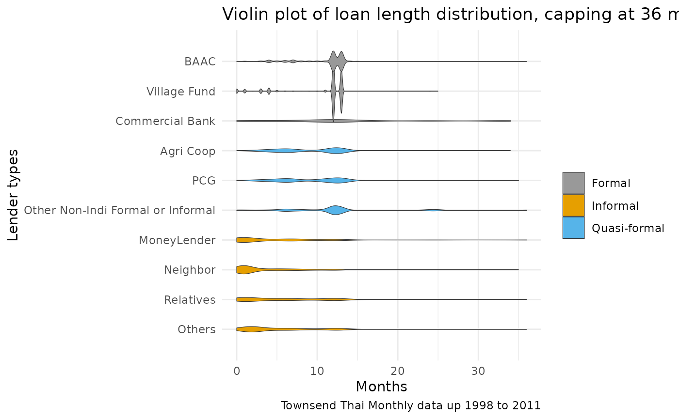
ffp_save_res_figure(pl_violin_loan_length_all, "pl_violin_loan_length_all", spt_res,
  bl_save = ls_save_res[["pl_violin_loan_length_all"]]
)
Loan length eight key categories
Loan length distribution among eight selected key categories.
First, in shares.
# We will first count the number of loans by type and month
pl_bar_loan_length_1a <- tstm_loans %>%
  ungroup() %>%
  filter(
    G_LenderType != "Other Non-Indi Formal or Informal",
    G_LenderType != "Commercial Bank",
  ) %>%
  group_by(forinfm3, G_LenderType, G_Loan_Init_Length) %>%
  summarize(group_len_count = n()) %>%
  ungroup() %>%
  group_by(forinfm3, G_LenderType) %>%
  mutate(group_count = sum(group_len_count)) %>%
  mutate(group_len_share = group_len_count / group_count) %>%
  filter(G_Loan_Init_Length <= 36) %>%
  ggplot(aes(
    x = G_Loan_Init_Length, y = group_len_share,
    fill = forinfm3, color = forinfm3
  )) +
  geom_bar(stat = "identity") +
  facet_wrap(factor(forinfm3, c(
    "Formal",
    "Quasi-formal",
    "Informal"
  )) ~
    factor(G_LenderType,
      levels = c(
        "MoneyLender",
        "Neighbor",
        "Relatives",
        "Others",
        "BAAC",
        "Village Fund",
        # 'Commercial Bank',
        "Agri Coop",
        "PCG"
      )
    ), scales = "free_y", ncol = 4) +
  scale_fill_manual(values = cbp1) +
  scale_color_manual(values = cbp1) +
  guides(color = FALSE, fill = FALSE) +
  theme_minimal() +
  labs(
    x = paste0("Number of months by which all principal + interests are due"),
    y = paste0("Share of loans with this duration"),
    title = paste(
      "Loan length distribution, capping at 36 months (share of loans)",
      sep = " "
    ),
    caption = paste(
      "Townsend Thai Monthly data up 1998 to 2011",
      sep = ""
    )
  )
#> `summarise()` has regrouped the output.
#> ℹ Summaries were computed grouped by forinfm3, G_LenderType, and
#>   G_Loan_Init_Length.
#> ℹ Output is grouped by forinfm3 and G_LenderType.
#> ℹ Use `summarise(.groups = "drop_last")` to silence this message.
#> ℹ Use `summarise(.by = c(forinfm3, G_LenderType, G_Loan_Init_Length))` for
#>   per-operation grouping (`?dplyr::dplyr_by`) instead.
#> Warning: The `<scale>` argument of `guides()` cannot be `FALSE`. Use "none" instead as
#> of ggplot2 3.3.4.
print(pl_bar_loan_length_1a)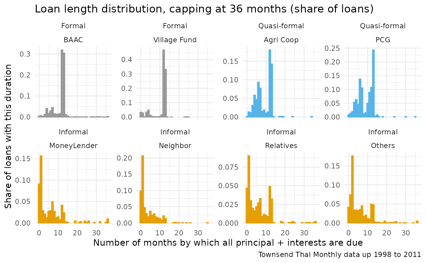
ffp_save_res_figure(pl_bar_loan_length_1a, "pl_bar_loan_length_1a", spt_res,
  bl_save = ls_save_res[["pl_bar_loan_length_1a"]]
)
Second, in levels (frequency of loans).
# We will first count the number of loans by type and month
pl_bar_loan_length_1b <- tstm_loans %>%
  ungroup() %>%
  filter(
    G_LenderType != "Other Non-Indi Formal or Informal",
    G_LenderType != "Commercial Bank",
  ) %>%
  group_by(forinfm3, G_LenderType, G_Loan_Init_Length) %>%
  summarize(group_len_count = n()) %>%
  ungroup() %>%
  group_by(forinfm3, G_LenderType) %>%
  mutate(group_count = sum(group_len_count)) %>%
  mutate(group_len_share = group_len_count / group_count) %>%
  filter(G_Loan_Init_Length <= 36) %>%
  ggplot(aes(
    x = G_Loan_Init_Length, y = group_len_count,
    fill = forinfm3, color = forinfm3
  )) +
  geom_bar(stat = "identity") +
  facet_wrap(factor(forinfm3, c(
    "Formal",
    "Quasi-formal",
    "Informal"
  )) ~
    factor(G_LenderType,
      levels = c(
        "MoneyLender",
        "Neighbor",
        "Relatives",
        "Others",
        "BAAC",
        "Village Fund",
        # 'Commercial Bank',
        "Agri Coop",
        "PCG"
      )
    ), scales = "free_y", ncol = 4) +
  scale_fill_manual(values = cbp1) +
  scale_color_manual(values = cbp1) +
  guides(color = FALSE, fill = FALSE) +
  theme_minimal() +
  labs(
    x = paste0("Number of months by which all principal + interests are due"),
    y = paste0("Number of loans with this duration"),
    title = paste(
      "Loan length distribution, capping at 36 months (number of loans)",
      sep = " "
    ),
    caption = paste(
      "Townsend Thai Monthly data up 1998 to 2011",
      sep = ""
    )
  )
#> `summarise()` has regrouped the output.
#> ℹ Summaries were computed grouped by forinfm3, G_LenderType, and
#>   G_Loan_Init_Length.
#> ℹ Output is grouped by forinfm3 and G_LenderType.
#> ℹ Use `summarise(.groups = "drop_last")` to silence this message.
#> ℹ Use `summarise(.by = c(forinfm3, G_LenderType, G_Loan_Init_Length))` for
#>   per-operation grouping (`?dplyr::dplyr_by`) instead.
print(pl_bar_loan_length_1b)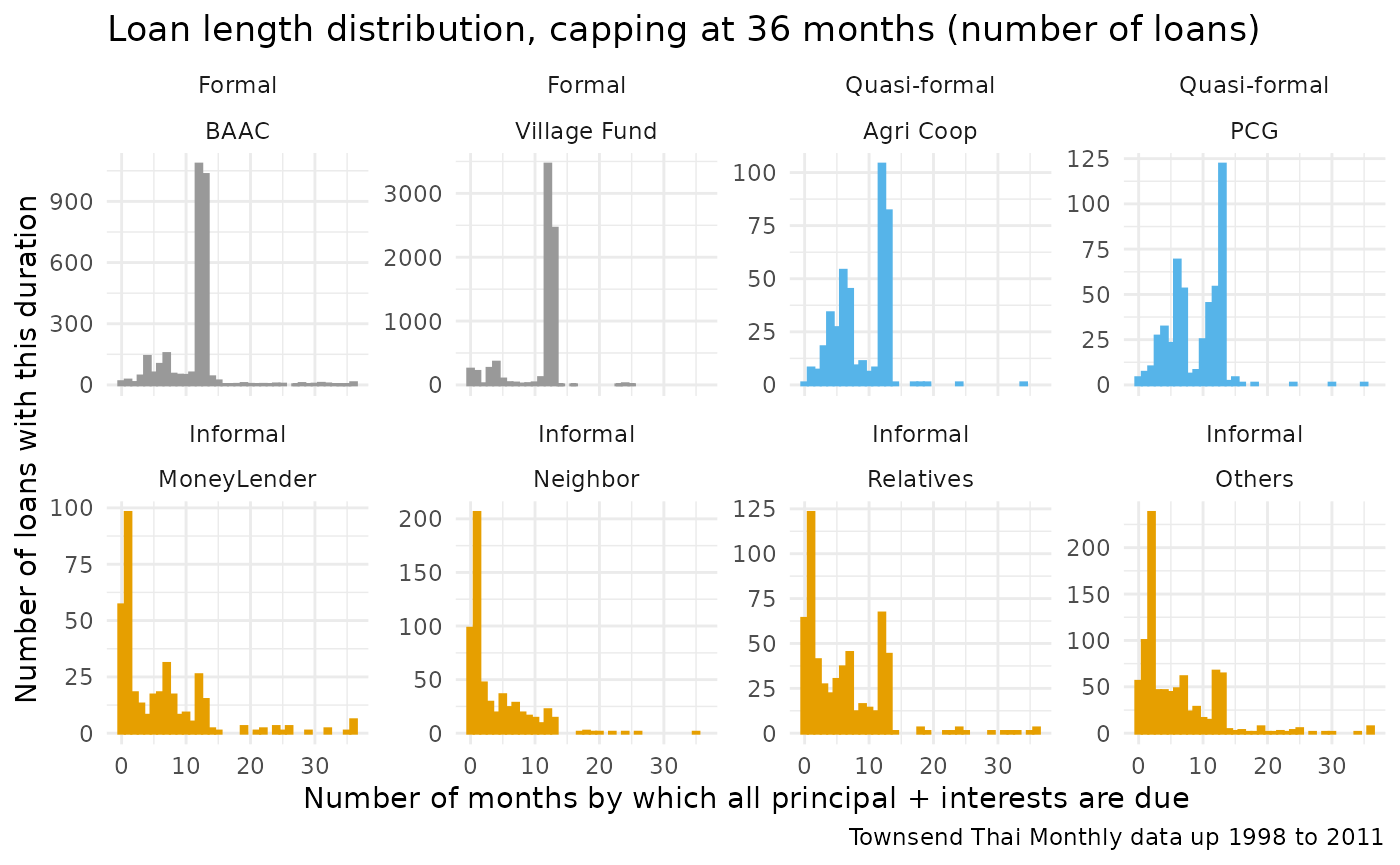
ffp_save_res_figure(pl_bar_loan_length_1b, "pl_bar_loan_length_1b", spt_res,
  bl_save = ls_save_res[["pl_bar_loan_length_1b"]]
)
Loan length three categories
Formal, informal, and quasi-formal laon length distribution break-down.
First, we visualize with share of loans (with just formal and informal, and with formal, informal, and quasiformal).
ar_it_forinf <- c(1, 2)
for (it_forinf in ar_it_forinf) {
  if (it_forinf == 1) {
    tstm_loans_use <- tstm_loans
  }
  if (it_forinf == 2) {
    tstm_loans_use <- tstm_loans %>% filter(forinfm3 != "Quasi-formal")
  }


  # We will first count the number of loans by type and month
  pl_bar_loan_length_2a_use <- tstm_loans_use %>%
    ungroup() %>%
    # filter(G_LenderType != "Other Non-Indi Formal or Informal",
    #        G_LenderType != "Commercial Bank",) %>%
    group_by(forinfm3, G_Loan_Init_Length) %>%
    summarize(group_len_count = n()) %>%
    ungroup() %>%
    group_by(forinfm3) %>%
    mutate(group_count = sum(group_len_count)) %>%
    mutate(group_len_share = group_len_count / group_count) %>%
    filter(G_Loan_Init_Length <= 24) %>%
    ggplot(aes(
      x = G_Loan_Init_Length, y = group_len_share,
      fill = forinfm3
    )) +
    geom_bar(stat = "identity") +
    facet_wrap(~ factor(forinfm3,
      levels = c(
        "Formal",
        "Quasi-formal",
        "Informal"
      )
    ), scales = "free_y", ncol = 3) +
    scale_fill_manual(values = cbp1) +
    scale_color_manual(values = cbp1) +
    guides(color = FALSE, fill = FALSE) +
    theme_minimal() +
    labs(
      x = paste0("Number of months by which all principal + interests are due"),
      y = paste0("Share of loans with this duration"),
      title = paste(
        "Loan length distribution, capping at 24 months (share of loans)",
        sep = " "
      ),
      caption = paste(
        "Townsend Thai Monthly data up 1998 to 2011",
        sep = ""
      )
    )
  print(pl_bar_loan_length_2a_use)

  if (it_forinf == 1) {
    pl_bar_loan_length_2a <- pl_bar_loan_length_2a_use
  }
  if (it_forinf == 2) {
    pl_bar_loan_length_2a_forinf <- pl_bar_loan_length_2a_use
  }
}
#> `summarise()` has regrouped the output.
#> ℹ Summaries were computed grouped by forinfm3 and G_Loan_Init_Length.
#> ℹ Output is grouped by forinfm3.
#> ℹ Use `summarise(.groups = "drop_last")` to silence this message.
#> ℹ Use `summarise(.by = c(forinfm3, G_Loan_Init_Length))` for per-operation
#>   grouping (`?dplyr::dplyr_by`) instead.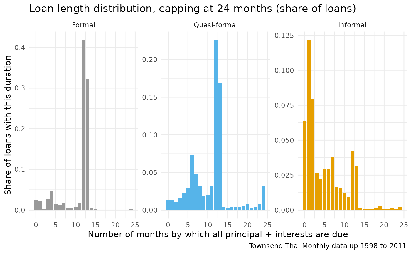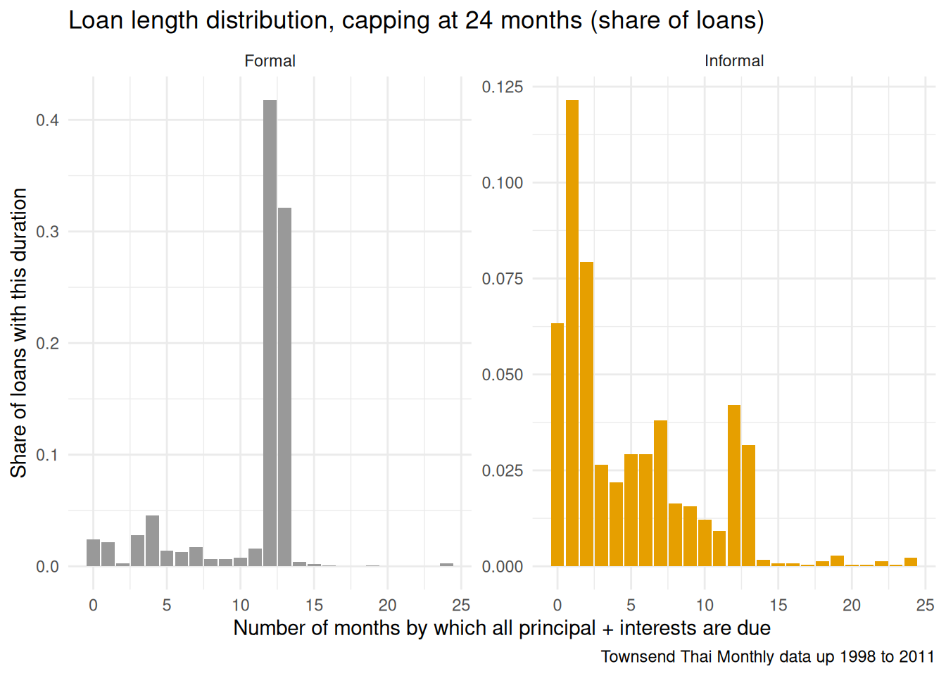
ffp_save_res_figure(pl_bar_loan_length_2a, "pl_bar_loan_length_2a", spt_res,
  bl_save = ls_save_res[["pl_bar_loan_length_2a"]]
)
ffp_save_res_figure(pl_bar_loan_length_2a_forinf, "pl_bar_loan_length_2a_forinf", spt_res,
  bl_save = ls_save_res[["pl_bar_loan_length_2a_forinf"]]
)
Second, we visualize with number of loans.
# Frequencies
pl_bar_loan_length_2b <- tstm_loans %>%
  ungroup() %>%
  # filter(G_LenderType != "Other Non-Indi Formal or Informal",
  #        G_LenderType != "Commercial Bank",) %>%
  group_by(forinfm3, G_Loan_Init_Length) %>%
  summarize(group_len_count = n()) %>%
  ungroup() %>%
  group_by(forinfm3) %>%
  mutate(group_count = sum(group_len_count)) %>%
  mutate(group_len_share = group_len_count / group_count) %>%
  filter(G_Loan_Init_Length <= 24) %>%
  ggplot(aes(
    x = G_Loan_Init_Length, y = group_len_count,
    fill = forinfm3
  )) +
  geom_bar(stat = "identity") +
  facet_wrap(~ factor(forinfm3,
    levels = c(
      "Formal",
      "Quasi-formal",
      "Informal"
    )
  ), scales = "free_y", ncol = 3) +
  scale_fill_manual(values = cbp1) +
  scale_color_manual(values = cbp1) +
  guides(color = FALSE, fill = FALSE) +
  theme_minimal() +
  labs(
    x = paste0("Number of months by which all principal + interests are due"),
    y = paste0("Number of loans with this duration"),
    title = paste(
      "Loan length distribution, capping at 24 months (number of loans)",
      sep = " "
    ),
    caption = paste(
      "Townsend Thai Monthly data up 1998 to 2011",
      sep = ""
    )
  )
#> `summarise()` has regrouped the output.
#> ℹ Summaries were computed grouped by forinfm3 and G_Loan_Init_Length.
#> ℹ Output is grouped by forinfm3.
#> ℹ Use `summarise(.groups = "drop_last")` to silence this message.
#> ℹ Use `summarise(.by = c(forinfm3, G_Loan_Init_Length))` for per-operation
#>   grouping (`?dplyr::dplyr_by`) instead.
print(pl_bar_loan_length_2b)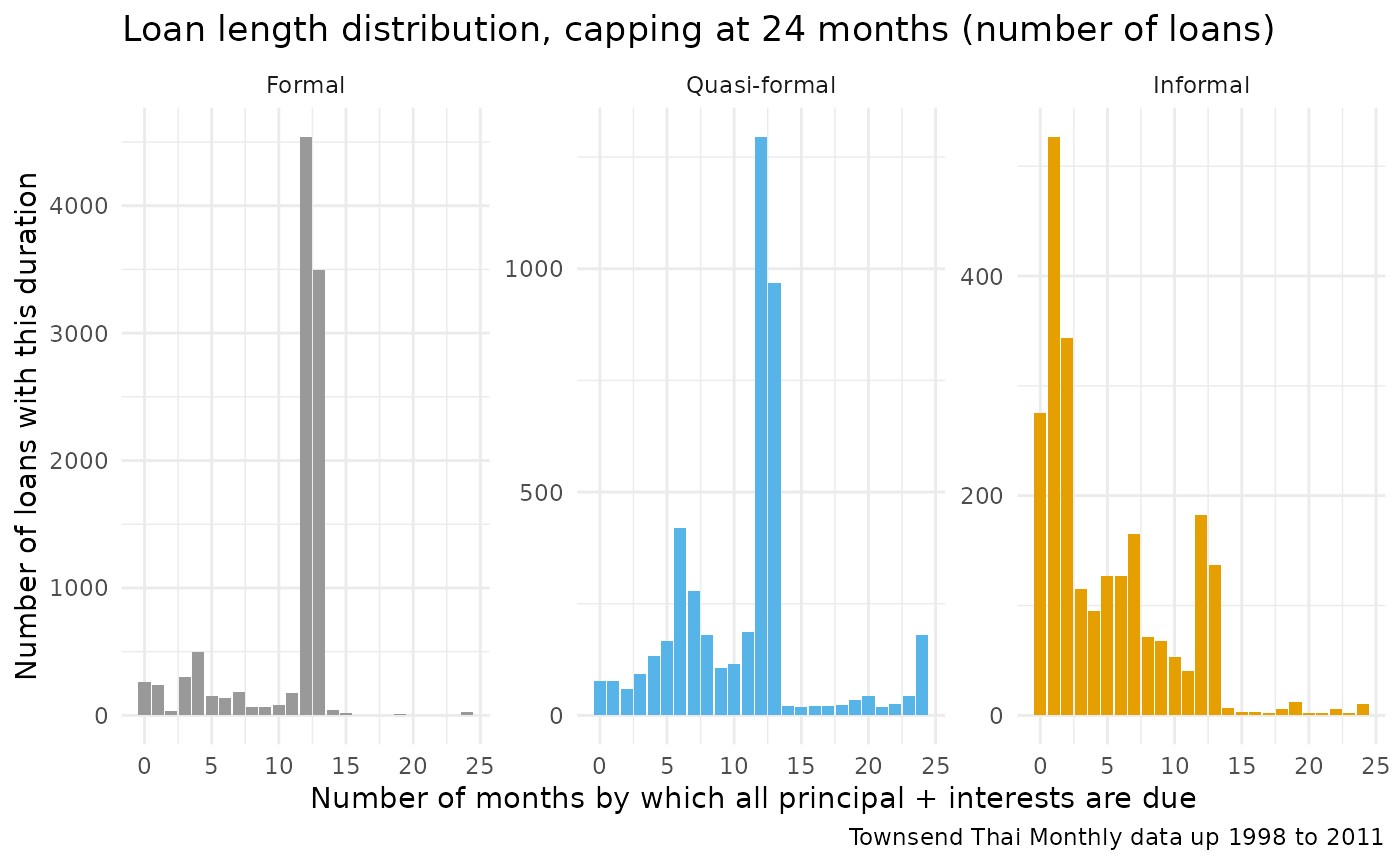
ffp_save_res_figure(pl_bar_loan_length_2b, "pl_bar_loan_length_2b", spt_res,
  bl_save = ls_save_res[["pl_bar_loan_length_2b"]]
)
Loan length overall formal and informal
First, fOrmal and informal, density plot.
# We will first count the number of loans by type and month
pl_bar_loan_length_3 <- tstm_loans %>%
  filter(G_Loan_Init_Length <= 36) %>%
  ggplot(aes(G_Loan_Init_Length,
    fill = formal, color = formal
  )) +
  geom_density(alpha = 0.5, stat = "density", position = "identity") +
  scale_fill_manual(values = cbp1) +
  scale_color_manual(values = cbp1) +
  guides(color = FALSE, fill = FALSE) +
  theme_minimal()
print(pl_bar_loan_length_3)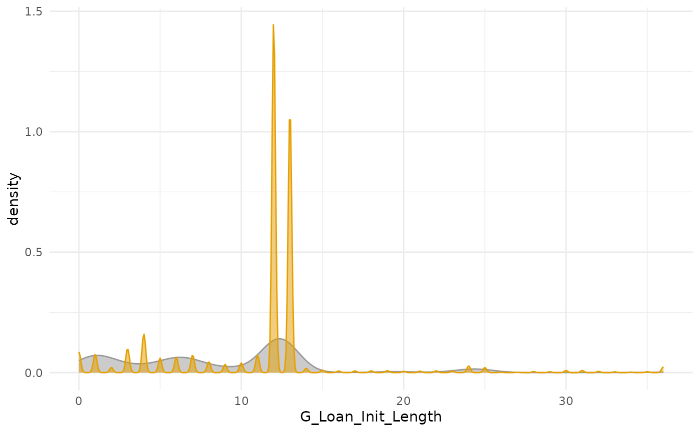
ffp_save_res_figure(pl_bar_loan_length_3, "pl_bar_loan_length_3", spt_res,
  bl_save = ls_save_res[["pl_bar_loan_length_3"]]
)
Second, formal vs informal bifurcation violin plot.
pl_loan_length <- tstm_loans %>%
  filter(G_Loan_Init_Length <= 36) %>%
  ggplot(aes(x = formal, y = G_Loan_Init_Length)) +
  geom_violin(
    width = 2.1, size = 0.2,
    fill = "#a4a4a4", color = "darkred"
  ) +
  theme_minimal() +
  coord_flip() +
  labs(
    y = paste0("Months"),
    x = paste0("Formal vs Informal"),
    title = paste(
      "Violin plot of loan length distribution, capping at 36 months",
      sep = " "
    ),
    caption = paste(
      "Townsend Thai Monthly data up 1998 to 2011",
      sep = ""
    )
  )
print(pl_loan_length)
#> Warning: `position_dodge()` requires non-overlapping x intervals.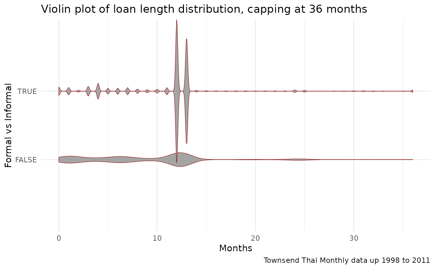
ffp_save_res_figure(pl_loan_length, "pl_loan_length", spt_res,
  bl_save = ls_save_res[["pl_loan_length"]]
)
Loan amount distribution
Loan amount all loan type violin plot
Overall and all types of lenders:
# Figure B: Loan Amount by Lender Types
pl_violin_loan_size_all <- tstm_loans %>%
  mutate(S_Init_Amount_Log = log(S_Init_Amount)) %>%
  # filter(G_Loan_Init_Length <= 24) %>%
  ggplot(aes(x = factor(G_LenderType,
    levels = rev(c(
      "BAAC",
      "Village Fund",
      "Commercial Bank",
      "Agri Coop",
      "PCG",
      "Other Non-Indi Formal or Informal",
      "MoneyLender",
      "Neighbor",
      "Relatives",
      "Others"
    ))
  ), y = S_Init_Amount_Log, fill = forinfm3)) +
  geom_violin(
    width = 2.1, size = 0.2,
  ) +
  scale_fill_manual(values = cbp1, name = "") +
  theme_minimal() +
  coord_flip() +
  labs(
    y = paste0("Natural log of loan size (amount in baht)"),
    x = paste0("Lender types"),
    title = paste(
      "Violin plot of log loan size (amount in Baht) distribution",
      sep = " "
    ),
    caption = paste(
      "Townsend Thai Monthly data up 1998 to 2011",
      sep = ""
    )
  )
print(pl_violin_loan_size_all)
#> Warning: Removed 12 rows containing non-finite outside the scale range
#> (`stat_ydensity()`).
#> Warning: `position_dodge()` requires non-overlapping x intervals.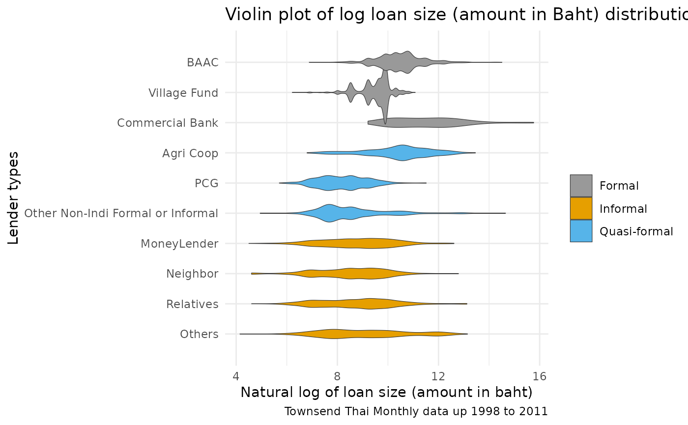
ffp_save_res_figure(pl_violin_loan_size_all, "pl_violin_loan_size_all", spt_res,
  bl_save = ls_save_res[["pl_violin_loan_size_all"]]
)
Loan amount key categories distributions
Compare eight key categories.
# # Density plot
# pl_loan_amount_density <- tstm_loans %>%
#   mutate(S_Init_Amount_Log = log(S_Init_Amount)) %>%
#   ggplot(aes(S_Init_Amount_Log,
#              fill=formal, color=formal)) +
#   geom_density(alpha=0.5, stat = "density", position = "identity") +
#   facet_wrap(~ G_LenderType + formal, scales = "free_y") +
#   theme_minimal()
# print(pl_loan_amount_density)
# Density plot
pl_loan_amount_density_1 <- tstm_loans %>%
  filter(
    G_LenderType != "Other Non-Indi Formal or Informal",
    G_LenderType != "Commercial Bank",
  ) %>%
  mutate(S_Init_Amount_Log = log(S_Init_Amount)) %>%
  ggplot(aes(S_Init_Amount_Log,
    fill = forinfm3, color = forinfm3
  )) +
  geom_density(alpha = 0.5, stat = "density", position = "identity") +
  facet_wrap(factor(forinfm3, c(
    "Formal",
    "Quasi-formal",
    "Informal"
  )) ~
    factor(G_LenderType,
      levels = c(
        "MoneyLender",
        "Neighbor",
        "Relatives",
        "Others",
        "BAAC",
        "Village Fund",
        # 'Commercial Bank',
        "Agri Coop",
        "PCG"
      )
    ), scales = "free_y", ncol = 4) +
  scale_fill_manual(values = cbp1) +
  scale_color_manual(values = cbp1) +
  guides(color = FALSE, fill = FALSE) +
  theme_minimal()
print(pl_loan_amount_density_1)
#> Warning: Removed 6 rows containing non-finite outside the scale range
#> (`stat_density()`).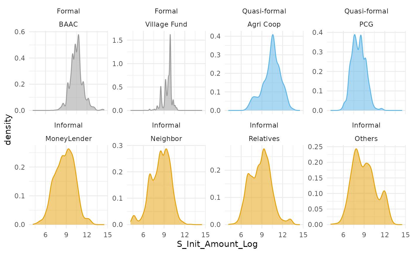
ffp_save_res_figure(pl_loan_amount_density_1, "pl_loan_amount_density_1", spt_res,
  bl_save = ls_save_res[["pl_loan_amount_density_1"]]
)
Compare distributions by formal and informal groupings, individual categories overlapping.
pl_loan_amount_density_2 <- tstm_loans %>%
  filter(
    G_LenderType != "Other Non-Indi Formal or Informal",
    G_LenderType != "Commercial Bank",
  ) %>%
  mutate(S_Init_Amount_Log = log(S_Init_Amount)) %>%
  ggplot(aes(S_Init_Amount_Log,
    fill = G_LenderType, color = G_LenderType
  )) +
  geom_density(alpha = 0.5, stat = "density", position = "identity") +
  facet_wrap(~formal, scales = "free_y", ncol = 1) +
  scale_fill_manual(values = cbp1) +
  scale_color_manual(values = cbp1) +
  theme_minimal()
print(pl_loan_amount_density_2)
#> Warning: Removed 6 rows containing non-finite outside the scale range
#> (`stat_density()`).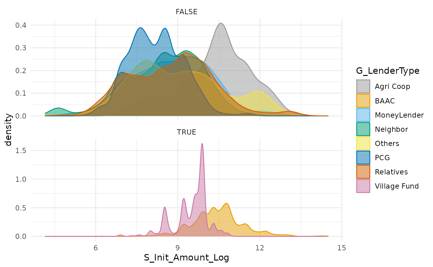
ffp_save_res_figure(pl_loan_amount_density_2, "pl_loan_amount_density_2", spt_res,
  bl_save = ls_save_res[["pl_loan_amount_density_2"]]
)
Loan amount formal vs informal vs quasi
ar_it_forinf <- c(1, 2)
for (it_forinf in ar_it_forinf) {
  if (it_forinf == 1) {
    tstm_loans_use <- tstm_loans
  }
  if (it_forinf == 2) {
    tstm_loans_use <- tstm_loans %>% filter(forinfm3 != "Quasi-formal")
  }

  pl_density_loan_size_forinfm3_use <- tstm_loans_use %>%
    mutate(S_Init_Amount_Log = log(S_Init_Amount)) %>%
    ggplot(aes(S_Init_Amount_Log,
      fill = forinfm3, color = forinfm3
    )) +
    geom_density(alpha = 0.5, stat = "density", position = "identity") +
    scale_fill_manual(values = cbp1, name = "") +
    scale_color_manual(values = cbp1, name = "") +
    theme_minimal() +
    labs(
      x = paste0("Natural log of loan size (amount in baht)"),
      y = paste0("Density"),
      title = paste(
        "Density of log loan size (amount in Baht) distribution",
        sep = " "
      ),
      caption = paste(
        "Townsend Thai Monthly data up 1998 to 2011",
        sep = ""
      )
    )
  print(pl_density_loan_size_forinfm3_use)

  if (it_forinf == 1) {
    pl_density_loan_size_forinfm3 <- pl_density_loan_size_forinfm3_use
  }
  if (it_forinf == 2) {
    pl_density_loan_size_forinfm2 <- pl_density_loan_size_forinfm3_use
  }
}
#> Warning: Removed 12 rows containing non-finite outside the scale range
#> (`stat_density()`).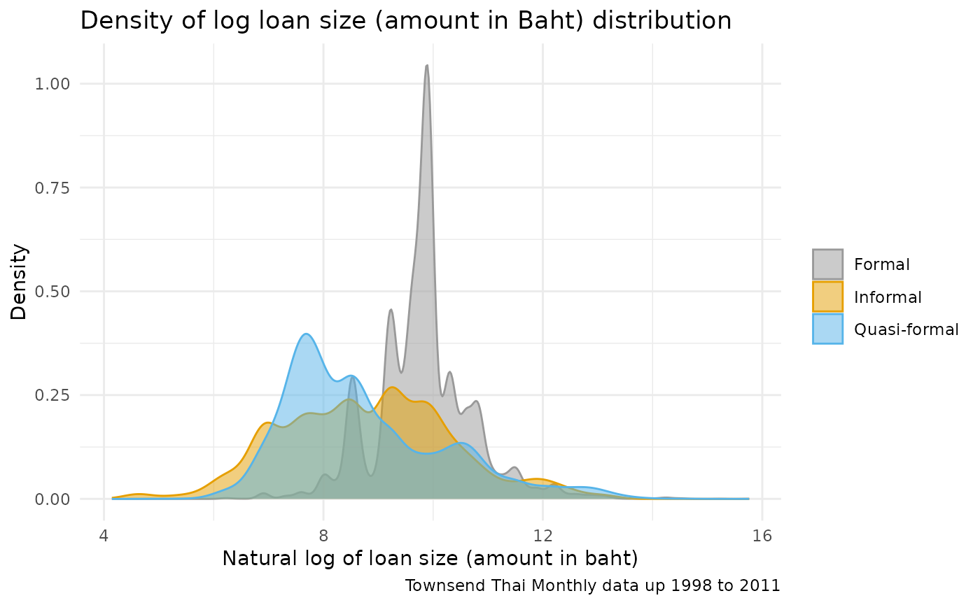
#> Warning: Removed 6 rows containing non-finite outside the scale range
#> (`stat_density()`).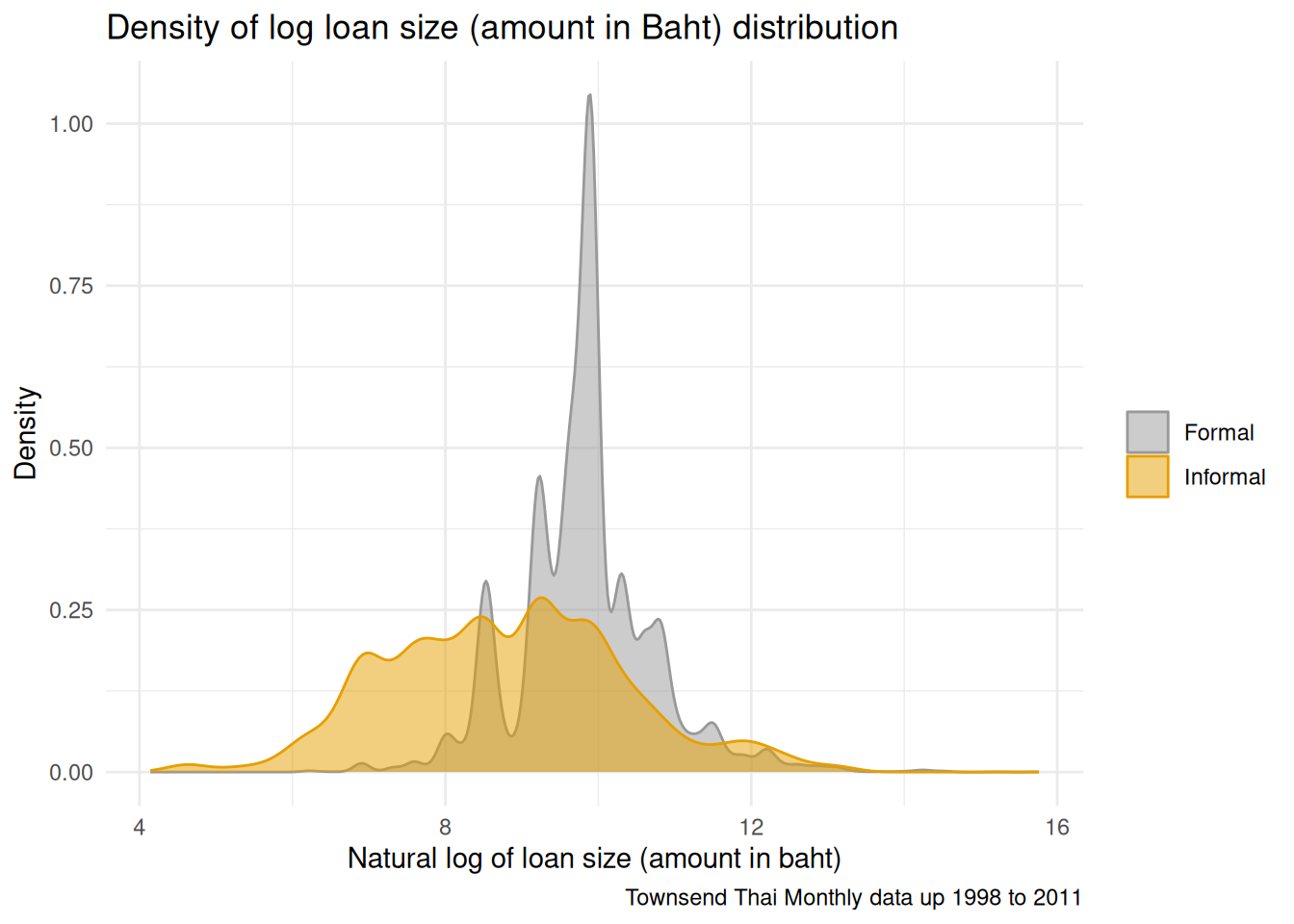
ffp_save_res_figure(pl_density_loan_size_forinfm3, "pl_density_loan_size_forinfm3", spt_res,
  bl_save = ls_save_res[["pl_density_loan_size_forinfm3"]]
)
ffp_save_res_figure(pl_density_loan_size_forinfm2, "pl_density_loan_size_forinfm2", spt_res,
  bl_save = ls_save_res[["pl_density_loan_size_forinfm2"]]
)
Loan amount formal vs informal distribution
Formal vs informal, density.
pl_density_loan_size_3 <- tstm_loans %>%
  mutate(S_Init_Amount_Log = log(S_Init_Amount)) %>%
  ggplot(aes(S_Init_Amount_Log,
    fill = formal, color = formal
  )) +
  geom_density(alpha = 0.5, stat = "density", position = "identity") +
  scale_fill_manual(values = cbp1) +
  scale_color_manual(values = cbp1) +
  theme_minimal() +
  labs(
    x = paste0("Natural log of loan size (amount in baht)"),
    y = paste0("Density"),
    title = paste(
      "Density of log loan size (amount in Baht) distribution",
      sep = " "
    ),
    caption = paste(
      "Townsend Thai Monthly data up 1998 to 2011",
      sep = ""
    )
  )
print(pl_density_loan_size_3)
#> Warning: Removed 12 rows containing non-finite outside the scale range
#> (`stat_density()`).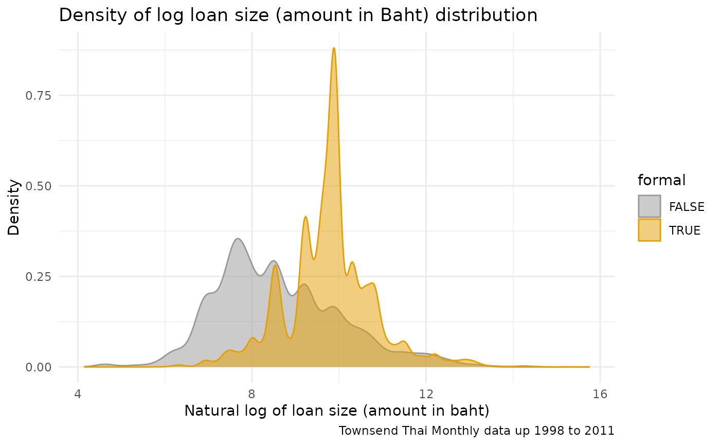
ffp_save_res_figure(pl_density_loan_size_3, "pl_density_loan_size_3", spt_res,
  bl_save = ls_save_res[["pl_density_loan_size_3"]]
)
Formal vs informal bifurcation, violin.
# Figure B: Loan Amount by Lender Types
pl_loan_size <- tstm_loans %>%
  mutate(S_Init_Amount_Log = log(S_Init_Amount)) %>%
  # filter(G_Loan_Init_Length <= 24) %>%
  ggplot(aes(x = formal, y = S_Init_Amount_Log)) +
  geom_violin(
    width = 2.1, size = 0.2,
    fill = "#A4A4A4", color = "darkred"
  ) +
  theme_minimal() +
  coord_flip() +
  labs(
    y = paste0("Natural log of loan size (amount in baht)"),
    x = paste0("Formal vs informal"),
    title = paste(
      "Violin plot: log loan size (amount in Baht) dist",
      sep = " "
    ),
    caption = paste(
      "Townsend Thai Monthly data up 1998 to 2011",
      sep = ""
    )
  )
print(pl_loan_size)
#> Warning: Removed 12 rows containing non-finite outside the scale range
#> (`stat_ydensity()`).
#> Warning: `position_dodge()` requires non-overlapping x intervals.
ffp_save_res_figure(pl_loan_size, "pl_loan_size", spt_res,
  bl_save = ls_save_res[["pl_loan_size"]]
)
Loan interest rate distribution
Interest rate all loan type violin plot
Overall and all types of lenders.
# Figure C: Interest Rate By Loan Types
pl_violin_loan_rate_all <- tstm_loans %>%
  mutate(
    G_Loan_Init_IntMthlyRat_Log =
      log((G_Loan_Init_IntMthlyRat) * 100 + 1)
  ) %>%
  filter(G_Loan_Init_IntMthlyRat_Log <= 3) %>%
  # filter(G_Loan_Init_IntMthlyRat <= 0.15) %>%
  ggplot(aes(x = factor(G_LenderType,
    levels = rev(c(
      "BAAC",
      "Village Fund",
      "Commercial Bank",
      "Agri Coop",
      "PCG",
      "Other Non-Indi Formal or Informal",
      "MoneyLender",
      "Neighbor",
      "Relatives",
      "Others"
    ))
  ), y = G_Loan_Init_IntMthlyRat_Log, fill = forinfm3)) +
  geom_violin(
    width = 2.1, size = 0.2
  ) +
  scale_fill_manual(values = cbp1, name = "") +
  theme_minimal() +
  coord_flip() +
  labs(
    y = paste0("Natural log of (monthly loan interest x 100 + 1)"),
    # y = paste0("Monthly loan interest"),
    x = paste0("Lender types"),
    title = paste(
      # "Monthly interest distribution (annual/weekly interest rates converted to monthly)",
      "Log of (monthly interest x 100 + 1) dist.\n",
      "Annual and weekly loan interest rates converted to monthly",
      sep = " "
    ),
    caption = paste(
      "Townsend Thai Monthly data up 1998 to 2011",
      sep = ""
    )
  )
print(pl_violin_loan_rate_all)
#> Warning: `position_dodge()` requires non-overlapping x intervals.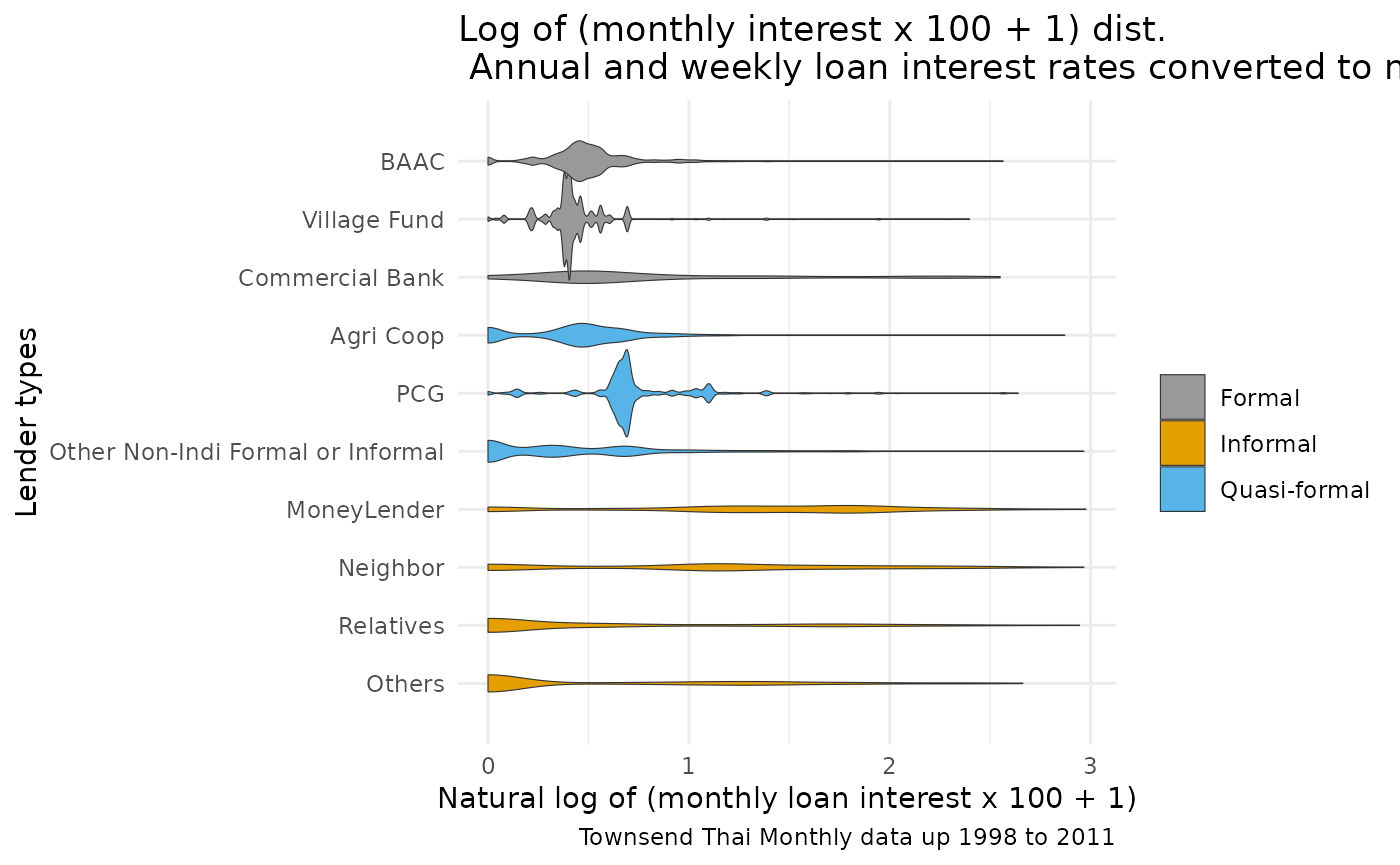
ffp_save_res_figure(pl_violin_loan_rate_all, "pl_violin_loan_rate_all", spt_res,
  bl_save = ls_save_res[["pl_violin_loan_rate_all"]]
)
Interest rate key categories distribution
Eight categories separate plots.
ar_it_forinf <- c(1, 2)
for (it_forinf in ar_it_forinf) {
  if (it_forinf == 1) {
    tstm_loans_use <- tstm_loans
  }
  if (it_forinf == 2) {
    tstm_loans_use <- tstm_loans %>% filter(forinfm3 != "Quasi-formal")
  }

  # Density plot
  pl_density_loan_rate_forinfm3_bym8_use <- tstm_loans_use %>%
    filter(
      G_LenderType != "Other Non-Indi Formal or Informal",
      G_LenderType != "Commercial Bank",
    ) %>%
    mutate(
      G_Loan_Init_IntMthlyRat_Log =
        log((G_Loan_Init_IntMthlyRat) * 100 + 1)
    ) %>%
    filter(G_Loan_Init_IntMthlyRat <= 0.15) %>%
    ggplot(aes(G_Loan_Init_IntMthlyRat,
      fill = forinfm3, color = forinfm3
    )) +
    geom_density(alpha = 0.5, stat = "density", position = "identity")

  if (it_forinf == 1) {
    pl_density_loan_rate_forinfm3_bym8_use <- pl_density_loan_rate_forinfm3_bym8_use +
      facet_wrap(factor(forinfm3, c(
        "Formal",
        "Quasi-formal",
        "Informal"
      )) ~ factor(G_LenderType,
        levels = c(
          "MoneyLender",
          "Neighbor",
          "Relatives",
          "Others",
          "BAAC",
          "Village Fund",
          # 'Commercial Bank',
          "Agri Coop",
          "PCG"
        )
      ), scales = "free_y", ncol = 4)
  }
  if (it_forinf == 2) {
    pl_density_loan_rate_forinfm3_bym8_use <- pl_density_loan_rate_forinfm3_bym8_use +
      facet_wrap(factor(forinfm3, c(
        "Informal",
        "Formal"
      )) ~ factor(G_LenderType,
        levels = c(
          "MoneyLender",
          "Neighbor",
          "Relatives",
          "Others",
          "BAAC",
          "Village Fund"
        )
      ), scales = "free_y", ncol = 4)
  }

  pl_density_loan_rate_forinfm3_bym8_use <- pl_density_loan_rate_forinfm3_bym8_use +
    scale_fill_manual(values = cbp1) +
    scale_color_manual(values = cbp1) +
    guides(color = FALSE, fill = FALSE) +
    theme_minimal() +
    labs(
      x = paste0("Monthly loan interest"),
      y = "Density",
      title = paste(
        "Monthly interest distribution (annual/weekly interest rates converted to monthly)",
        sep = " "
      ),
      caption = paste(
        "Townsend Thai Monthly data up 1998 to 2011",
        sep = ""
      )
    )
  print(pl_density_loan_rate_forinfm3_bym8_use)

  if (it_forinf == 1) {
    pl_density_loan_rate_forinfm3_bym8 <- pl_density_loan_rate_forinfm3_bym8_use
  }
  if (it_forinf == 2) {
    pl_density_loan_rate_forinfm3_bym8_forinf <- pl_density_loan_rate_forinfm3_bym8_use
  }
}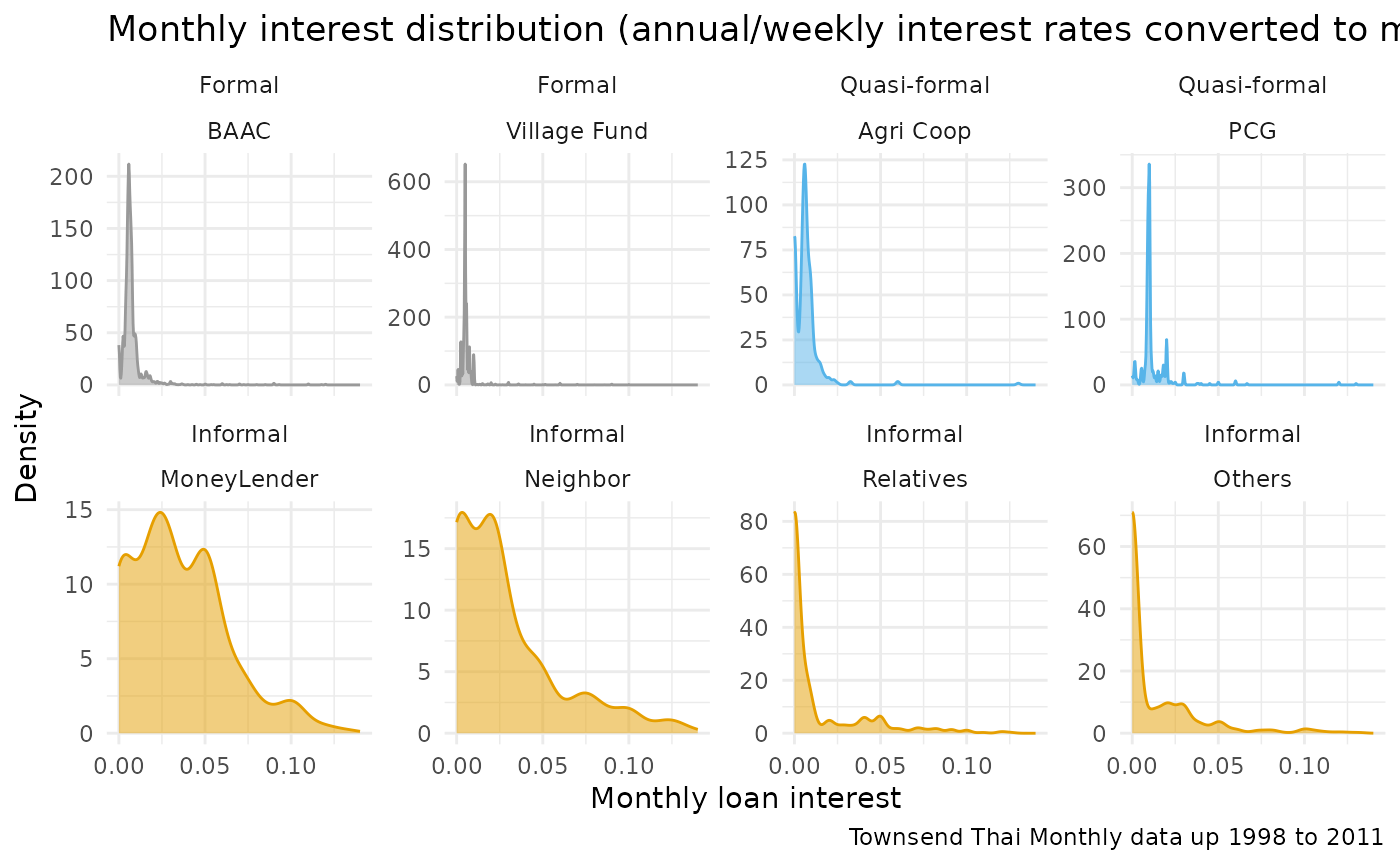
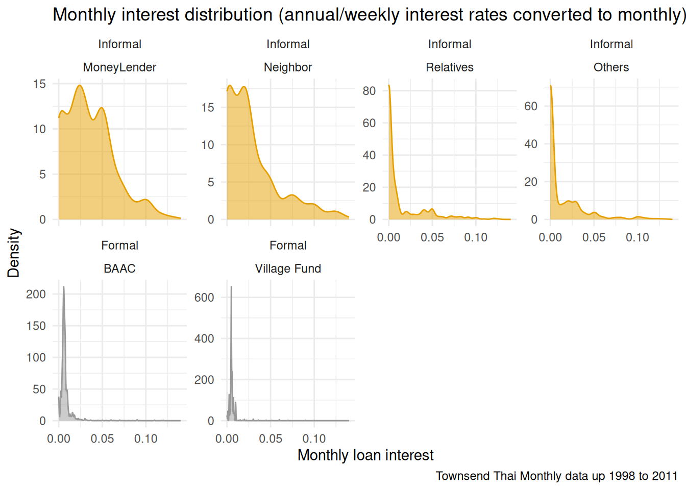
ffp_save_res_figure(pl_density_loan_rate_forinfm3_bym8, "pl_density_loan_rate_forinfm3_bym8", spt_res,
  bl_save = ls_save_res[["pl_density_loan_rate_forinfm3_bym8"]]
)
ffp_save_res_figure(pl_density_loan_rate_forinfm3_bym8_forinf, "pl_density_loan_rate_forinfm3_bym8_forinf", spt_res,
  bl_save = ls_save_res[["pl_density_loan_rate_forinfm3_bym8_forinf"]]
)
Overlapping distributions grouped by formal and informal.
# Density plot
pl_density_loan_rate_2 <- tstm_loans %>%
  filter(
    G_LenderType != "Other Non-Indi Formal or Informal",
    G_LenderType != "Commercial Bank",
  ) %>%
  mutate(
    G_Loan_Init_IntMthlyRat_Log =
      log((G_Loan_Init_IntMthlyRat) * 100 + 1)
  ) %>%
  filter(G_Loan_Init_IntMthlyRat <= 0.15) %>%
  ggplot(aes(G_Loan_Init_IntMthlyRat_Log,
    fill = G_LenderType, color = G_LenderType
  )) +
  geom_density(alpha = 0.5, stat = "density", position = "identity") +
  # facet_wrap(~ institutional + G_LenderType, scales = "free_y") +
  facet_wrap(~formal, scales = "free_y", ncol = 1) +
  scale_fill_manual(values = cbp1) +
  scale_color_manual(values = cbp1) +
  theme_minimal()
print(pl_density_loan_rate_2)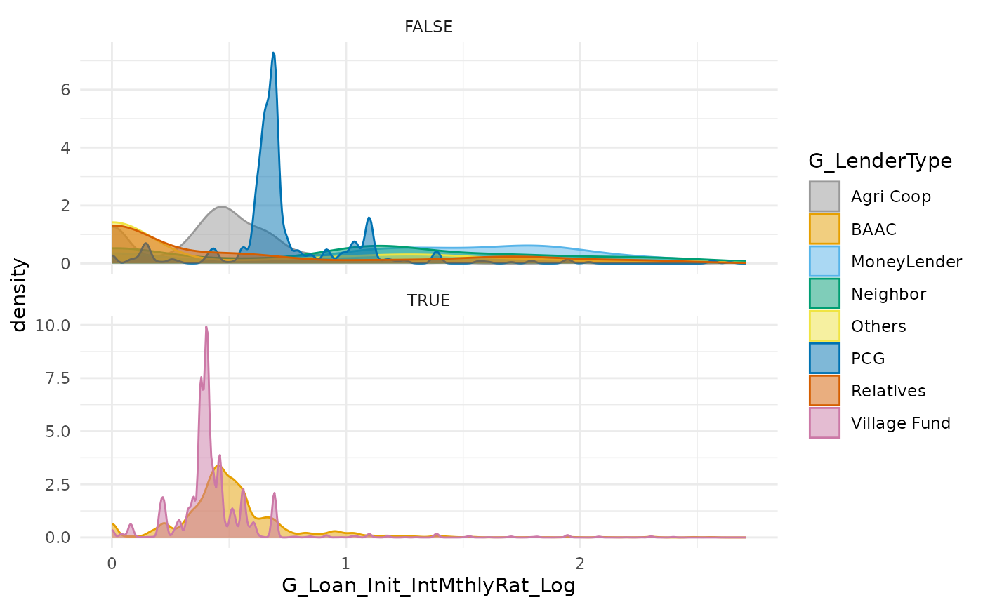
ffp_save_res_figure(pl_density_loan_rate_2, "pl_density_loan_rate_2", spt_res,
  bl_save = ls_save_res[["pl_density_loan_rate_2"]]
)
Interest rate formal vs informal vs quasi
# Density plot,
pl_density_loan_rate_4 <- tstm_loans %>%
  filter(G_Loan_Init_IntMthlyRat <= 0.15) %>%
  ggplot(aes(G_Loan_Init_IntMthlyRat,
    fill = forinfm3, color = forinfm3
  )) +
  geom_density(alpha = 0.5, stat = "density", position = "identity") +
  scale_fill_manual(values = cbp1) +
  scale_color_manual(values = cbp1) +
  theme_minimal()
print(pl_density_loan_rate_4)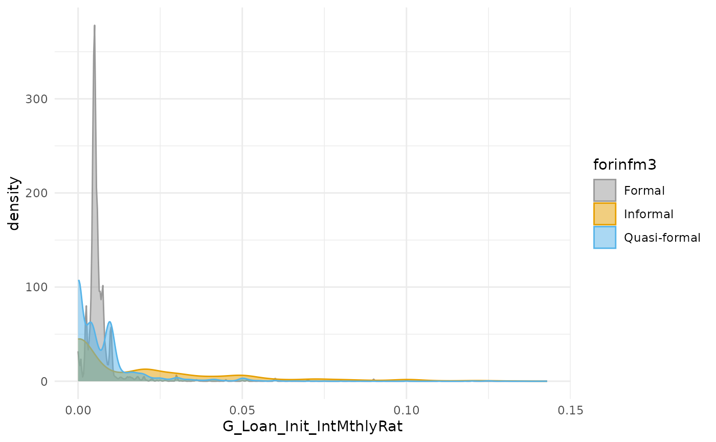
ffp_save_res_figure(pl_density_loan_rate_4, "pl_density_loan_rate_4", spt_res,
  bl_save = ls_save_res[["pl_density_loan_rate_4"]]
)
Interest rate formal vs informal
Formal vs informal density.
# Density plot
pl_density_loan_rate_3 <- tstm_loans %>%
  mutate(
    G_Loan_Init_IntMthlyRat_Log =
      log((G_Loan_Init_IntMthlyRat) * 100 + 1)
  ) %>%
  filter(G_Loan_Init_IntMthlyRat_Log <= 3) %>%
  ggplot(aes(G_Loan_Init_IntMthlyRat_Log,
    fill = formal, color = formal
  )) +
  geom_density(alpha = 0.5, stat = "density", position = "identity") +
  scale_fill_manual(values = cbp1) +
  scale_color_manual(values = cbp1) +
  theme_minimal()
print(pl_density_loan_rate_3)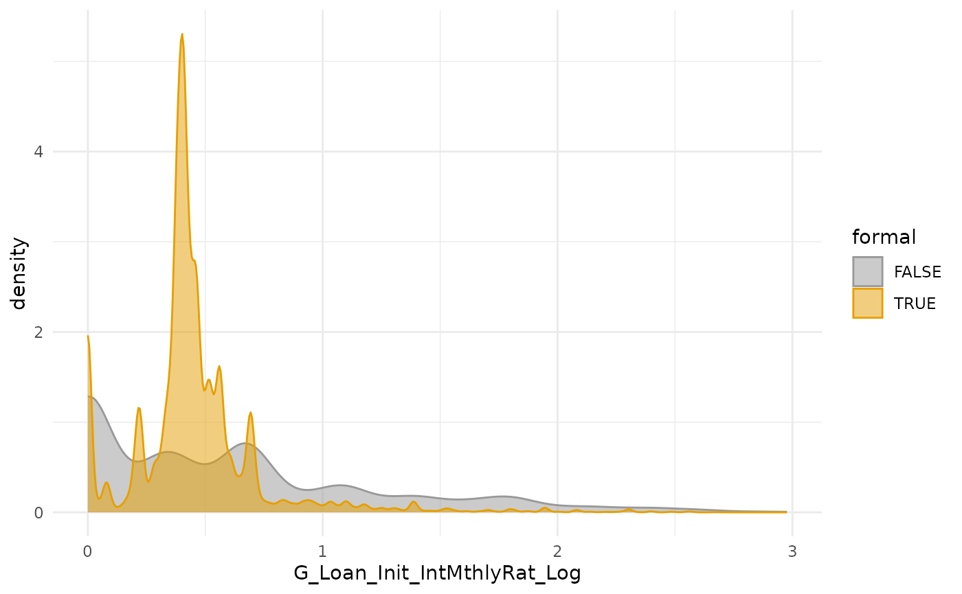
ffp_save_res_figure(pl_density_loan_rate_3, "pl_density_loan_rate_3", spt_res,
  bl_save = ls_save_res[["pl_density_loan_rate_3"]]
)
Formal vs informal bifurcation via violin plots.
# Figure C: Interest Rate By Loan Types
pl_loan_rate <- tstm_loans %>%
  mutate(
    G_Loan_Init_IntMthlyRat_Log =
      log((G_Loan_Init_IntMthlyRat) * 100 + 1)
  ) %>%
  filter(G_Loan_Init_IntMthlyRat_Log <= 3) %>%
  ggplot(aes(x = formal, y = G_Loan_Init_IntMthlyRat_Log)) +
  geom_violin(
    width = 2.1, size = 0.2,
    fill = "#A4A4A4", color = "darkred"
  ) +
  theme_minimal() +
  coord_flip() +
  labs(
    y = paste0("Natural log of (monthly loan interest x 100 + 1)"),
    x = paste0("Formal vs informal"),
    title = paste(
      "Violin plot: log of (monthly interest x 100 + 1) dist.\n",
      "Annual and weekly loan interest rates converted to monthly",
      sep = " "
    ),
    caption = paste(
      "Townsend Thai Monthly data up 1998 to 2011",
      sep = ""
    )
  )
print(pl_loan_rate)
#> Warning: `position_dodge()` requires non-overlapping x intervals.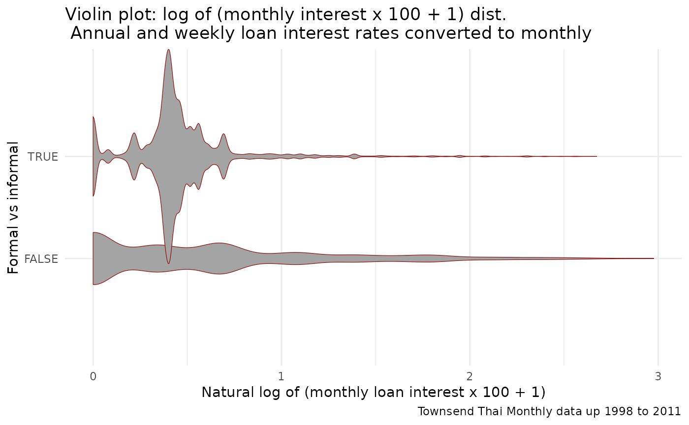
ffp_save_res_figure(pl_loan_rate, "pl_loan_rate", spt_res,
  bl_save = ls_save_res[["pl_loan_rate"]]
)
Saving Figures
Tables and figures are written to the package res/res_loan_terms_dist folder by the inline ffp_save_res_table() / ffp_save_res_figure() calls above, controlled per output by ls_save_res (all default to FALSE).