Chapter 5 Estimation
5.1 Linear Estimation
5.1.1 Linear OLS Regression
Go back to fan’s MEconTools Package, Matlab Code Examples Repository (bookdown site), or Math for Econ with Matlab Repository (bookdown site).
5.1.1.1 Fit a Line through Origin to Two Points
Fit a line from the origin through two points, given Equations \(Y=a\cdot X\), where we have two pairs of points for x and y.
rng(3);
[x1, x2] = deal(rand(),rand());
[y1, y2] = deal(rand(),rand());
ar_x = [x1,x2]';
ar_y = [y1,y2]';
Fit a line through the two points, passing through the x-intercept. Three formulas that provide the same answer.
% simple formula
fl_slope_basic = (1/(x1*x1 + x2*x2))*(x1*y1 + x2*y2);
% (X'X)^(-1)(X'Y)
fl_slope_matrix = inv(ar_x'*ar_x)*(ar_x'*ar_y);
% Use matlab function
tb_slope_fitlm = fitlm(ar_x, ar_y, 'Intercept',false);
fl_slope_fitlm = tb_slope_fitlm.Coefficients{1, 1};
Visualize results.
figure();
hold on;
scatter([x1,x2], [y1,y2]);
xlim([0, 1]);
ylim([0, 1]);
refline(fl_slope_basic, 0);
grid on;
grid minor;
title('Best fit line through origin with two points');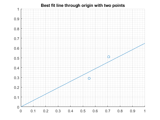
5.1.1.2 Exactly Identify Three Linear Equations with Three Unknown Parameters
We have three "observations" equations with three unknown \(\beta\) parameters, Generate the true \(y\) value based on random right-hand-side matrix and true \(\beta\), and estimate/solve for \(\beta\) given "data" on \(y\) and \(x\) matrix.
First generate the data.
% Generate a 3 by 3 matrix of random values
rng(3);
it_row_n = 3;
it_col_n = 3;
mt_rhs = rand([it_row_n, it_col_n]);

% Generate true coefficients
ar_beta_true = rand([it_row_n, 1]);

% Generate LHS, given true parameter
ar_lhs = mt_rhs*ar_beta_true;
Second, the estimating/exact-fit equation and estimated/solved \(\beta\).
% OLS regression function
fc_ols_lin = @(y, x) (x'*x)^(-1)*(x'*y);

% Estimate
ar_beta_esti = fc_ols_lin(ar_lhs, mt_rhs);

% Display
tb_beta = array2table([ar_beta_true, ar_beta_esti]);
cl_col_names = ["beta true", "beta estimates"];
cl_row_names = strcat('row_coef_', string((1:it_row_n)));
tb_beta.Properties.VariableNames = matlab.lang.makeValidName(cl_col_names);
tb_beta.Properties.RowNames = matlab.lang.makeValidName(cl_row_names);
disp(tb_beta);

                  betaTrue    betaEstimates
                  ________    _____________

    row_coef_1     0.44081       0.44081
    row_coef_2    0.029876      0.029876
    row_coef_3     0.45683       0.45683
5.2 Nonlinear Estimation
5.2.1 Nonlinear Estimation with Fminunc
Go back to fan’s MEconTools Package, Matlab Code Examples Repository (bookdown site), or Math for Econ with Matlab Repository (bookdown site).
5.2.1.1 Nonlinear Estimation Inputs LHS and RHS
Estimate this equation: \(\omega_t =\left(\nu_0 +a_0 \right)+a_1 t-\log \left(1-\exp \left(a_0 +a_1 t\right)\right)+\nu_t\). We have data from multiple \(t\), and want to estimate the \(a_0\), and \(a_1\) coefficients mainly, but also \(\nu_0\) is good as well. This is an estimation problem with 3 unknowns. \(t\) ranges from
% LHS outcome variable
ar_w = [-1.7349,-1.5559,-1.4334,-1.3080,-1.1791,-1.0462,-0.9085,-0.7652,-0.6150,-0.4564,-0.2874,-0.1052,0.0943];
% RHS t variable
ar_t = [0,3,5,7,9,11,13,15,16,19,21,23,25];
% actual parameters, estimation checks if gets actual parameters back
ar_a = [-1.8974, 0.0500];
5.2.1.2 Prediction and MSE Equations
Objective function for prediction and mean-squared-error.
v_0 = 0.5;
obj_ar_predictions = @(a) (v_0 + a(1) + a(2).*ar_t - log(1 - exp(a(1) + a(2).*ar_t)));
obj_fl_mse = @(a) mean((obj_ar_predictions(a) - ar_w).^2);
Evaluate given ar_a vectors.
ar_predict_at_actual = obj_ar_predictions(ar_a);
fl_mse_at_actual = obj_fl_mse(ar_a);
mt_compare = [ar_w', ar_predict_at_actual'];
tb_compare = array2table(mt_compare);
tb_compare.Properties.VariableNames = {'lhs-outcomes', 'evaluate-rhs-at-actual-parameters'};
disp(tb_compare);

    lhs-outcomes    evaluate-rhs-at-actual-parameters
    ____________    _________________________________

      -1.7349                    -1.2349
      -1.5559                     -1.056
      -1.4334                   -0.93353
       -1.308                   -0.80813
      -1.1791                   -0.67928
      -1.0462                   -0.54641
      -0.9085                   -0.40877
      -0.7652                   -0.26546
       -0.615                   -0.19133
      -0.4564                   0.043211
      -0.2874                    0.21214
      -0.1052                    0.39429
       0.0943                    0.59369
5.2.1.3 Unconstrained Nonlinear Estimation
Estimation to minimize mean-squared-error.
% Estimation options
options = optimset('display','on');
% Starting values
ar_a_init = [-10, -10];
% Optimize
[ar_a_opti, fl_fval] = fminunc(obj_fl_mse, ar_a_init, options);

Local minimum found.

Optimization completed because the size of the gradient is less than
the value of the optimality tolerance.

<stopping criteria details>
Compare results.
mt_compare = [ar_a_opti', ar_a'];
tb_compare = array2table(mt_compare);
tb_compare.Properties.VariableNames = {'estimated-best-fit', 'actual-parameters'};
disp(tb_compare);

    estimated-best-fit    actual-parameters
    __________________    _________________

          -2.3541              -1.8974
         0.057095                 0.05