Chapter 4 Simulation
4.1 Normal Distribution
4.1.1 Compute CDF for Normal and Bivariate Normal Distributions
Go back to fan’s MEconTools Package, Matlab Code Examples Repository (bookdown site), or Math for Econ with Matlab Repository (bookdown site).
CDF for normal random variable through simulation and with NORMCDF function. CDF for bivariate normal random variables through simulation and with NORMCDF function.
4.1.1.1 Simulate Normal Distribution Probability with Uniform Draws
Mean score is 0, standard deviation is 1, we want to know what is the chance that children score less than -2, -1, 0, 1, and 2 respectively. We have a solution to the normal CDF cumulative distribution problem, it is:
mu = 0;
sigma = 1;
ar_x = [-2,-1,0,1,2];
for x=ar_x
    cdf_x = normcdf(x, mu, sigma);
    disp([strjoin(...
        ["CDF with normcdf", ...
        ['x=' num2str(x)] ...
        ['cdf_x=' num2str(cdf_x)] ...
        ], ";")]);
end

CDF with normcdf;x=-2;cdf_x=0.02275
CDF with normcdf;x=-1;cdf_x=0.15866
CDF with normcdf;x=0;cdf_x=0.5
CDF with normcdf;x=1;cdf_x=0.84134
CDF with normcdf;x=2;cdf_x=0.97725
We can also approximate the probabilities above, by drawing many points from a unifom:
Draw from uniform distribution 0 to 1, N times.
Invert these using invnorm. This means our uniform draws are now effectively drawn from the normal distribution.
Check if each draw inverted is below the x threshold or above, count fractions.
We should get very similar results as in the example above (especially if N is large)
% set seed
rng(123);
% generate random numbers
N = 10000;
ar_unif_draws = rand(1,N);
% invert
ar_normal_draws = norminv(ar_unif_draws);
% loop over different x values
for x=ar_x
    % index if draws below x
    ar_it_idx_below_x = (ar_normal_draws < x);
    fl_frac_below_x = (sum(ar_it_idx_below_x))/N;
    disp([strjoin(...
        ["CDF with normcdf", ...
        ['x=' num2str(x)] ...
        ['fl_frac_below_x=' num2str(fl_frac_below_x)] ...
        ], ";")]);
end

CDF with normcdf;x=-2;fl_frac_below_x=0.023
CDF with normcdf;x=-1;fl_frac_below_x=0.1612
CDF with normcdf;x=0;fl_frac_below_x=0.4965
CDF with normcdf;x=1;fl_frac_below_x=0.847
CDF with normcdf;x=2;fl_frac_below_x=0.9789
4.1.1.2 Simulate Bivariate-Normal Distribution Probability with Uniform Draws
There are two tests now, a math test and an English test. Student test scores are correlated with correlation 0.5 from the two tests, mean and standard deviations are 0 and 1 for both tests. What is the chance that a student scores below -2 and -2 for both, below -2 and 0 for math and English, below 2 and 1 for math and English, etc?
% timer
tm_start_mvncdf = tic;
% mean, and varcov
ar_mu = [0,0];
mt_varcov = [1,0.5;0.5,1];
ar_x = linspace(-3,3,101);
% initialize storage
mt_prob_math_eng = zeros([length(ar_x), length(ar_x)]);
% loop over math and english score thresholds
it_math = 0;
for math=ar_x
    it_math = it_math + 1;
    it_eng = 0;
    for eng=ar_x
        it_eng = it_eng + 1;
        % points below which to compute probability
        ar_scores = [math, eng];
        % volumn of a mountain to the southwest of north-south and east-west cuts
        cdf_x = mvncdf(ar_scores, ar_mu, mt_varcov);
        mt_prob_math_eng(it_math, it_eng) = cdf_x;
    end
end
% end timer
tm_end_mvncdf = toc(tm_start_mvncdf);
st_complete = strjoin(...
    ["MVNCDF Completed CDF computes", ...
     ['number of points=' num2str(numel(mt_prob_math_eng))] ...
     ['time=' num2str(tm_end_mvncdf)] ...
    ], ";");
disp(st_complete);

MVNCDF Completed CDF computes;number of points=10201;time=1.1957

% show results
tb_prob_math_eng = array2table(round(mt_prob_math_eng, 4));
cl_col_names_a = strcat('english <=', string(ar_x'));
cl_row_names_a = strcat('math <=', string(ar_x'));
tb_prob_math_eng.Properties.VariableNames = cl_col_names_a;
tb_prob_math_eng.Properties.RowNames = cl_row_names_a;
% subsetting function
% https://fanwangecon.github.io/M4Econ/amto/array/htmlpdfm/fs_slicing.html#19_Given_Array_of_size_M,_Select_N_somewhat_equi-distance_elements
f_subset = @(it_subset_n, it_ar_n) unique(round(((0:1:(it_subset_n-1))/(it_subset_n-1))*(it_ar_n-1)+1));
disp(tb_prob_math_eng(f_subset(7, length(ar_x)), f_subset(7, length(ar_x))));

                    english <=-3    english <=-1.98    english <=-1.02    english <=0    english <=1.02    english <=1.98    english <=3
                    ____________    _______________    _______________    ___________    ______________    ______________    ___________

    math <=-3          0.0001           0.0005              0.001           0.0013           0.0013            0.0013          0.0013
    math <=-1.98       0.0005           0.0043             0.0136           0.0217           0.0237            0.0238          0.0239
    math <=-1.02        0.001           0.0136             0.0598           0.1239           0.1505            0.1537          0.1539
    math <=0           0.0013           0.0217             0.1239           0.3333           0.4701            0.4978             0.5
    math <=1.02        0.0013           0.0237             0.1505           0.4701           0.7521            0.8359          0.8458
    math <=1.98        0.0013           0.0238             0.1537           0.4978           0.8359            0.9566          0.9753
    math <=3           0.0013           0.0239             0.1539              0.5           0.8458            0.9753          0.9974
We can also approximate the probabilities above, by drawing many points from two iid uniforms, and translating them to correlated normal using cholesky decomposition:
Draw from two random uniform distribution 0 to 1, N times each
Invert these using invnorm for both iid vectors from unifom draws to normal draws
Choleskey decompose and multiplication
This method below is faster than the method above when the number of points where we have to evaluat probabilities is large.
Generate randomly drawn scores:
% timer
tm_start_chol = tic;
% Draws uniform and invert to standard normal draws
N = 10000;
rng(123);
ar_unif_draws = rand(1,N*2);
ar_normal_draws = norminv(ar_unif_draws);
ar_draws_eta_1 = ar_normal_draws(1:N);
ar_draws_eta_2 = ar_normal_draws((N+1):N*2);

% Choesley decompose the variance covariance matrix
mt_varcov_chol = chol(mt_varcov, 'lower');

% Generate correlated random normals
mt_scores_chol = ar_mu' + mt_varcov_chol*([ar_draws_eta_1; ar_draws_eta_2]);
ar_math_scores = mt_scores_chol(1,:)';
ar_eng_scores = mt_scores_chol(2,:)';
Approximate probabilities from randomly drawn scores:
% initialize storage
mt_prob_math_eng_approx = zeros([length(ar_x), length(ar_x)]);
% loop over math and english score thresholds
it_math = 0;
for math=ar_x
    it_math = it_math + 1;
    it_eng = 0;
    for eng=ar_x
        it_eng = it_eng + 1;

        % points below which to compute probability
        % index if draws below x
        ar_it_idx_below_x_math = (ar_math_scores < math);
        ar_it_idx_below_x_eng = (ar_eng_scores < eng);
        ar_it_idx_below_x_joint = ar_it_idx_below_x_math.*ar_it_idx_below_x_eng;
        fl_frac_below_x_approx = (sum(ar_it_idx_below_x_joint))/N;

        % volumn of a mountain to the southwest of north-south and east-west cuts
        mt_prob_math_eng_approx(it_math, it_eng) = fl_frac_below_x_approx;
    end
end
% end timer
tm_end_chol = toc(tm_start_chol);
st_complete = strjoin(...
    ["UNIF+CHOL Completed CDF computes", ...
     ['number of points=' num2str(numel(mt_prob_math_eng_approx))] ...
     ['time=' num2str(tm_end_chol)] ...
    ], ";");
disp(st_complete);

UNIF+CHOL Completed CDF computes;number of points=10201;time=0.28661

% show results
tb_prob_math_eng_approx = array2table(round(mt_prob_math_eng_approx, 4));
cl_col_names_a = strcat('english <=', string(ar_x'));
cl_row_names_a = strcat('math <=', string(ar_x'));
tb_prob_math_eng_approx.Properties.VariableNames = cl_col_names_a;
tb_prob_math_eng_approx.Properties.RowNames = cl_row_names_a;
disp(tb_prob_math_eng_approx(f_subset(7, length(ar_x)), f_subset(7, length(ar_x))));

                    english <=-3    english <=-1.98    english <=-1.02    english <=0    english <=1.02    english <=1.98    english <=3
                    ____________    _______________    _______________    ___________    ______________    ______________    ___________

    math <=-3          0.0001           0.0005              0.001           0.0016           0.0016            0.0016          0.0016
    math <=-1.98       0.0003            0.004             0.0132           0.0218           0.0237            0.0239          0.0239
    math <=-1.02       0.0008           0.0131              0.061           0.1272           0.1529             0.157          0.1571
    math <=0           0.0009           0.0202             0.1236            0.334           0.4661            0.4946          0.4965
    math <=1.02        0.0009           0.0215             0.1493           0.4724            0.754            0.8411          0.8511
    math <=1.98        0.0009           0.0217             0.1526           0.4989           0.8344            0.9591           0.977
    math <=3           0.0009           0.0217             0.1526           0.5007           0.8425            0.9768          0.9976
4.1.2 Cholesky Decomposition Correlated Bivariate Normal from IID Random Draws
Go back to fan’s MEconTools Package, Matlab Code Examples Repository (bookdown site), or Math for Econ with Matlab Repository (bookdown site).
Draw two correlated normal shocks using the MVNRND function. Draw two correlated normal shocks from uniform random variables using Cholesky Decomposition.
4.1.2.1 Positively Correlated Scores MVNRND
We have English and Math scores, and we draw from a bivariate normal distribution, assuming the two scores are positively correlatd. These are \(x_1\) and \(x_2\).
% mean, and varcov
ar_mu = [70,80];
mt_varcov = [8,5;5,5];
% Generate Scores
rng(123);
N = 10000;
mt_scores = mvnrnd(ar_mu, mt_varcov, N);
% graph
figure();
scatter(mt_scores(:,1), mt_scores(:,2));
ylabel('English Scores');
xlabel('Math Scores')
grid on;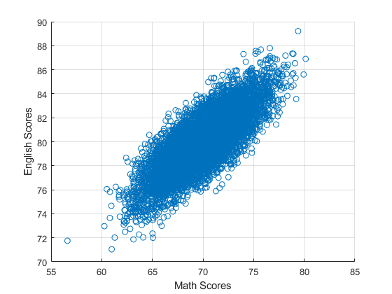
What are the covariance and correlation statistics?
disp([num2str(cov(mt_scores(:,1), mt_scores(:,2)))]);

8.0557      5.0738
5.0738      5.0638

disp([num2str(corrcoef(mt_scores(:,1), mt_scores(:,2)))]);

      1     0.79441
0.79441           1
4.1.2.2 Bivariate Normal from Uncorrelated Draws via Cholesky Decomposition
We can get the same results as above, without having to explicitly draw from a multivariate distribution by (For more details see Train (2009)):
Draw 2 uniform random iid vectors.
Convert to normal iid vectors.
Generate the test scores as a function of the two random variables, using Cholesky matrix.
First, draw two uncorrelated normal random variables, with mean 0, sd 1, \(\eta_1\) and \(\eta_2\).
% Draw Two Uncorrelated Normal Random Variables
% use the same N as above
rng(123);
% uniform draws, uncorrelated
ar_unif_draws = rand(1,N*2);
% normal draws, english and math are uncorreated
% ar_draws_eta_1 and ar_draws_eta_2 are uncorrelated by construction
ar_normal_draws = norminv(ar_unif_draws);
ar_draws_eta_1 = ar_normal_draws(1:N);
ar_draws_eta_2 = ar_normal_draws((N+1):N*2);
% graph
figure();
scatter(ar_draws_eta_1, ar_draws_eta_2);
ylabel('iid eta 1 draws');
xlabel('iid eta 2 draws')
grid on;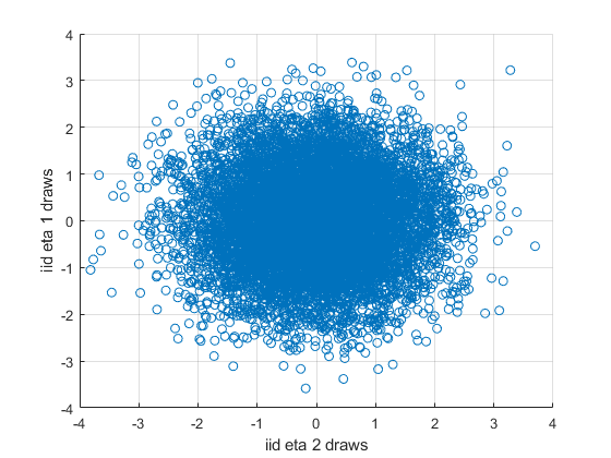
% Show Mean 1, cov = 0
disp([num2str(cov(ar_draws_eta_1, ar_draws_eta_2))]);

  0.99075   0.0056929
0.0056929     0.98517

disp([num2str(corrcoef(ar_draws_eta_1, ar_draws_eta_2))]);

        1   0.0057623
0.0057623 1Second, now using the variance-covariance we already have, decompose it, we will have:
- \(\displaystyle \begin{array}{l} c_{aa} \,,\,\,0\\ c_{ab} \,,\,\,c_{bb} \end{array}\)
% Choesley decompose the variance covariance matrix
mt_varcov_chol = chol(mt_varcov, 'lower');
disp([num2str(mt_varcov_chol)]);

2.8284           0
1.7678      1.3693

% The cholesky decomposed matrix factorizes the original varcov matrix
disp([num2str(mt_varcov_chol*mt_varcov_chol')]);

8           5
5 5Third, We can get back to the original \(x_1\) and \(x_2\) variables:
\(\displaystyle x_1 =\mu_1 +c_{aa} *\eta_1\)
\(\displaystyle x_2 =\mu_2 +c_{ab} *\eta_1 +c_{bb} *\eta_2\)
% multiple the cholesky matrix by the eta draws
mt_scores_chol = ar_mu' + mt_varcov_chol*([ar_draws_eta_1; ar_draws_eta_2]);
mt_scores_chol = mt_scores_chol';
% graph
figure();
scatter(mt_scores_chol(:,1), mt_scores_chol(:,2));
ylabel('English Scores Chol from iid Draws = m1 + c\_aa*eta\_1');
xlabel('Math Scores Chol from iid Draws = m2 + c\_ab*eta\_1 + c\_bb*eta\_2')
grid on;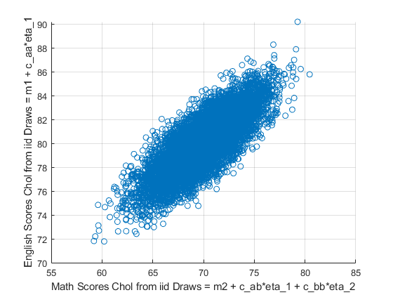
disp([num2str(cov(mt_scores_chol(:,1), mt_scores_chol(:,2)))]);

 7.926      4.9758
4.9758      4.9708

disp([num2str(corrcoef(mt_scores_chol(:,1), mt_scores_chol(:,2)))]);

      1     0.79272
0.79272           1
4.1.3 Cholesky Decomposition Correlated Five Dimensional Multivariate Normal Shock
Go back to fan’s MEconTools Package, Matlab Code Examples Repository (bookdown site), or Math for Econ with Matlab Repository (bookdown site).
Generate variance-covariance matrix from correlation and standard deviation. Draw five correlated normal shocks using the MVNRND function. Draw five correlated normal shocks from uniform random variables using Cholesky Decomposition.
4.1.3.1 Correlation and Standard Deviations to Variance Covariance Matrix
Given correlations and standard deviations, what is the variance and covariance matrix? Assume mean 0. The first three variables are correlated, the final two are iid.
First the ingredients:
% mean array
ar_mu = [0,0,0,0,0];
% standard deviations
ar_sd = [0.3301, 0.3329, 0.3308, 2312, 13394];
% correlations
mt_cor = ...
    [1,0.1226,0.0182,0,0;...
     0.1226,1,0.4727,0,0;...
     0.0182,0.4727,1,0,0;...
     0,0,0,1,0;...
     0,0,0,0,1];
% show
disp(mt_cor);

    1.0000    0.1226    0.0182         0         0
    0.1226    1.0000    0.4727         0         0
    0.0182    0.4727    1.0000         0         0
         0         0         0    1.0000         0
         0         0         0         0    1.0000
Second, we know that variance is the square of standard deviation. And we know the formula for covariance, which is variance divided by two standard deviations. So for the example here, we have:
% initialize
mt_varcov = zeros([5,5]);
% variance
mt_varcov(eye(5)==1) = ar_sd.^2;
% covariance
mt_varcov(1,2) = mt_cor(1,2)*ar_sd(1)*ar_sd(2);
mt_varcov(2,1) = mt_varcov(1,2);
mt_varcov(1,3) = mt_cor(1,3)*ar_sd(1)*ar_sd(3);
mt_varcov(3,1) = mt_varcov(1,3);
mt_varcov(2,3) = mt_cor(2,3)*ar_sd(2)*ar_sd(3);
mt_varcov(3,2) = mt_varcov(2,3);
% show
disp(mt_varcov(1:3,1:3));

    0.1090    0.0135    0.0020
    0.0135    0.1108    0.0521
    0.0020    0.0521    0.1094

disp(mt_varcov(4:5,4:5));

     5345344           0
           0   179399236
4.1.3.2 Draw Five Correlated Shocks Using MVNRND
Generate N5 correlated shock structure
% Generate Scores
rng(123);
N = 50000;
mt_kw97_eps = mvnrnd(ar_mu, mt_varcov, N);
% graph
figure();
% subfigure 1
subplot(2,2,1);
scatter(mt_kw97_eps(:,1), mt_kw97_eps(:,2));
ylabel('White Collar Wage Shock');
xlabel('Blue Collar Wage Shock')
grid on;
% subfigure 2
subplot(2,2,2);
scatter(mt_kw97_eps(:,1), mt_kw97_eps(:,3));
ylabel('White Collar Wage Shock');
xlabel('Military Wage Shock')
grid on;
% subfigure 3
subplot(2,2,3);
scatter(mt_kw97_eps(:,3), mt_kw97_eps(:,2));
ylabel('Military Wage Shock');
xlabel('Blue Collar Wage Shock')
grid on;
% subfigure 4
subplot(2,2,4);
scatter(mt_kw97_eps(:,1), mt_kw97_eps(:,4));
ylabel('White Collar Wage Shock');
xlabel('School Shock')
grid on;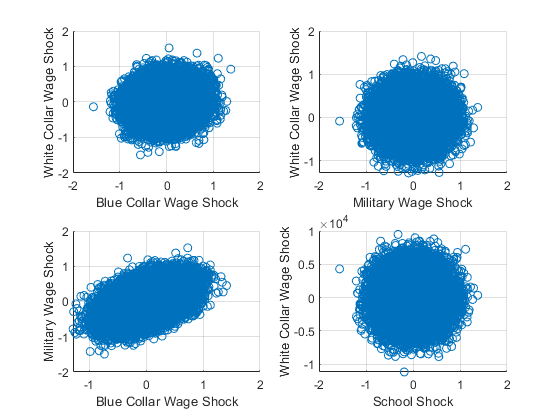
What are the covariance and correlation statistics?
disp([num2str(round(corrcoef(mt_kw97_eps),3))]);

     1       0.119       0.016       0.002      -0.003
 0.119           1       0.468      -0.003       0.004
 0.016       0.468           1      -0.003       0.001
 0.002      -0.003      -0.003           1      -0.005
-0.003       0.004       0.001      -0.005           1

disp([num2str(round(corrcoef(mt_kw97_eps),2))]);

   1        0.12        0.02           0           0
0.12           1        0.47           0           0
0.02        0.47           1           0           0
   0           0           0           1       -0.01
   0           0           0       -0.01           1
4.1.3.3 Draw Five Correlated Shocks Using Cholesky Decomposition
Following what we did for bivariate normal distribution, we can now do the same for five different shocks at the same time (For more details see Train (2009)):
Draw 5 normal random variables that are uncorrelated
Generate 5 correlated shocks
Draw the shocks
% Draws uniform and invert to standard normal draws
rng(123);
ar_unif_draws = rand(1,N*5);
ar_normal_draws = norminv(ar_unif_draws);
ar_draws_eta_1 = ar_normal_draws((N*0+1):N*1);
ar_draws_eta_2 = ar_normal_draws((N*1+1):N*2);
ar_draws_eta_3 = ar_normal_draws((N*2+1):N*3);
ar_draws_eta_4 = ar_normal_draws((N*3+1):N*4);
ar_draws_eta_5 = ar_normal_draws((N*4+1):N*5);

% Choesley decompose the variance covariance matrix
mt_varcov_chol = chol(mt_varcov, 'lower');

% Generate correlated random normals
mt_kp97_eps_chol = ar_mu' + mt_varcov_chol*([...
    ar_draws_eta_1; ar_draws_eta_2; ar_draws_eta_3; ar_draws_eta_4; ar_draws_eta_5]);
mt_kp97_eps_chol = mt_kp97_eps_chol';
Graph:
% graph
figure();
% subfigure 1
subplot(2,2,1);
scatter(mt_kp97_eps_chol(:,1), mt_kp97_eps_chol(:,2));
ylabel('CHOL White Collar Wage Shock');
xlabel('CHOL Blue Collar Wage Shock')
grid on;
% subfigure 2
subplot(2,2,2);
scatter(mt_kp97_eps_chol(:,1), mt_kp97_eps_chol(:,3));
ylabel('CHOL White Collar Wage Shock');
xlabel('CHOL Military Wage Shock')
grid on;
% subfigure 3
subplot(2,2,3);
scatter(mt_kp97_eps_chol(:,3), mt_kp97_eps_chol(:,2));
ylabel('CHOL Military Wage Shock');
xlabel('CHOL Blue Collar Wage Shock')
grid on;
% subfigure 4
subplot(2,2,4);
scatter(mt_kp97_eps_chol(:,1), mt_kp97_eps_chol(:,4));
ylabel('CHOL White Collar Wage Shock');
xlabel('CHOL School Shock')
grid on;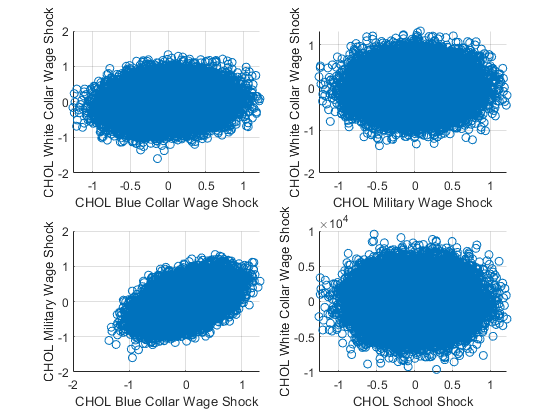
What are the covariance and correlation statistics?
disp([num2str(round(corrcoef(mt_kp97_eps_chol),3))]);

     1       0.119       0.021       0.008      -0.003
 0.119           1       0.479       0.008      -0.003
 0.021       0.479           1       0.002           0
 0.008       0.008       0.002           1      -0.004
-0.003      -0.003           0      -0.004           1

disp([num2str(round(corrcoef(mt_kp97_eps_chol),2))]);

   1        0.12        0.02        0.01           0
0.12           1        0.48        0.01           0
0.02        0.48           1           0           0
0.01        0.01           0           1           0
   0           0           0           0           1