Chapter 2 Commonly Used Functions
2.1 Exponentiation and Compounding Interest Rate
Go back to fan’s MEconTools Package, Matlab Code Examples Repository (bookdown site), or Math for Econ with Matlab Repository (bookdown site).
See also: Exponential Function and Log Function.
2.1.1 Exponential Function
Exopential Function: Functions where the variable \(x\) appears as an exponent: \(a^x\)
\(a\) is the base of Exponential function.
Remember that
\(\displaystyle a^0 =1\)
\(\displaystyle a^{\frac{1}{2}} =\sqrt{a}\)
if \(a^b =c\), we can also write, \(a=c^{\frac{1}{b}}\), for example, \(2^3 =8\), and \(2=8^{\frac{1}{3}}\)
\(\displaystyle a^{-b} =\frac{1}{a^b }\)
\(\displaystyle x^a \cdot x^b =x^{a+b}\)
\(\displaystyle x^{a\cdot b} =(x^a )^b\)
2.1.2 Exponential Function Graphs?
Note that the domain of exponential function includes positive and negative \(x\), and the exponential function will always be positive.
If base is below \(1\), then the curve is monotonically downward sloping
If base is above \(1\), then the curve is monotonically upwards sloping
If base is above \(1\), higher base leads to steeper curvature.
syms x
a1 = 0.5;
f_a1 = a1^(x);
a2 = 1.5;
f_a2 = a2^(x);
a3 = 2.5;
f_a3 = a3^(x);
figure();
hold on;
fplot(f_a1, [-2, 2]);
fplot(f_a2, [-2, 2]);
fplot(f_a3, [-2, 2]);
line([0,0],ylim);
line(xlim, [0,0]);
title('Exponential Function Graph with different bases')
legend(['base=',num2str(a1)], ['base=',num2str(a2)],['base=',num2str(a3)]);
grid on;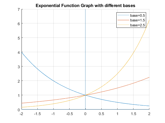
2.1.3 Infinitely Compounding Interest rate
with 100 percent interest rate (APR), if we compound \(N\) times within a year, interest we pay at the end of the year is
- \(\displaystyle (1+\frac{1}{N})^N -1\)
Suppose \(N=5\) (You can also think of this as a loan with interest rate of \(20\)% for every \(73\) days), then we pay \(159\)% interest rate by the end of the year.
r = 1.05;
N = 5;
(1 + r/N)^N - 1

ans = 1.5937
What if we do more and more compounding, if we say interest rate compounds \(10\), \(50\), \(100\) times over the year, what happens? With APR at 100%, the total interest rate you pay at the end of the year does not go to infinity, rather, it converges to this special number \(e\), Euler’s number, \(2.7182818\). This means if every second the interest rate is compounding, with an APR of 100%, you end up paying 272% of what you borrowed by the end of the year, which is 172% interest rate.
- \(\displaystyle \lim_{N\to \inf } (1+\frac{1}{N})^N =e\approx 2.7182818\)
We can visualize this limit below
r = 1;
syms N
f_compoundR = (1 + r/N)^N;
figure();
fplot(f_compoundR, [1,100])
ylabel({'Principle and Interests at End of Year Given 100% APR' 'for 1 dollar Borrowed, given infinite compounding'})
xlabel('Number of Evenly-divided Times to Compound Interest Rate in a Year')
grid on;
grid minor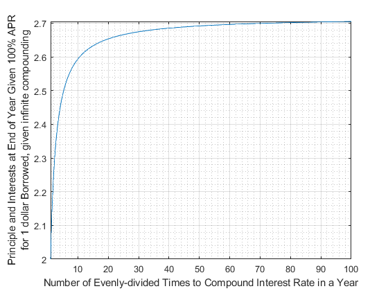
double(subs(f_compoundR,[1,2,3,4,5,6,7,8,9,10]))

ans = 1x10
    2.0000    2.2500    2.3704    2.4414    2.4883    2.5216    2.5465    2.5658    2.5812    2.5937
2.1.4 Infinitely compounding Interest rate, different \(r\) (APR \(r\))
Given:
- \(\displaystyle \lim_{N\to \inf } (1+\frac{1}{N})^N =e\approx 2.7182818\)
What is
- \(\lim_{N\to \inf } (1+\frac{r}{N})^N\)?
We can replace \(N\) by \(N=r\cdot M\)
- \(\displaystyle \lim_{N\to \inf } (1+\frac{r}{N})^N =\lim_{M\to \inf } (1+\frac{r}{r\cdot M})^{r\cdot M} ={\left(\lim_{M\to \inf } (1+\frac{1}{M})^M \right)}^r =e^r\)
This gives the base \(e\) exponential function a financial interpretation.
syms x
f_e = exp(x);
figure();
hold on;
fplot(f_e, [-3, 3]);
line([0,0],ylim);
line(xlim, [0,0]);
title('Exponential Function Graph with base e')
xlabel('r = interest rate');
ylabel({'Principle and Interests at End of Year' 'for 1 dollar Borrowed, given infinite compounding'})
grid on;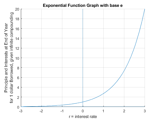
2.2 Natural Logarithm and Exponential
Go back to fan’s MEconTools Package, Matlab Code Examples Repository (bookdown site), or Math for Econ with Matlab Repository (bookdown site).
We use log for log utility in our household maximization problems, and we use exponential functions with other bases for production functions.
See also: Exponential and Infinitely Compounding Interest Rate.
2.2.1 Log and Exponential
If the natural log of \(x\) is \(y\) (in economics we generally just write ln and log interchangeably, becareful though, google thinks function log means log with base 10, matlab thinks function log means base e, you will get different numbers typing in log(10) in google and matlab).
- \(\displaystyle \ln (x)=y\)
then
- \(\displaystyle e^y =x\)
where e is Euler’s number. Intuitively, \(ln(x)\) is asking what exponent \(y\) of base \(e\) is needed for \(e^y\) to be equal to \(x\). When \(x\) is consumption, the log utility of consumption is in some sense the number of \(e\) terms needed to be multiplied together to equal to \(c\).
We can also write:
- \(e^x =\exp (x)\), writing \(\exp (x)\) is a little easier to read, means just \(e\) to the power of \(x\)
because of this:
since \(e^0 =1\), \(\log (1)=0\)
since \(e^1 \approx 2.71828\), \(\log (2.71828)\approx 1\)
The natural log is just the inverse of the exponential function. We use log to linearize exponential functions, which allows us to do regressions afterwards for example.
2.2.2 Log Rules
Suppose we have: \(\log \left(\frac{\exp (A+\epsilon )\cdot a^{\alpha } \cdot b^{\beta } }{c^{\theta } \cdot d^{\phi } }\right)\)
This looks complicated, but because there is log, we can take the equation apart:
\[\log \left(\frac{\exp (A+\epsilon )\cdot a^{\alpha } \cdot b^{\beta } }{c^{\theta } \cdot d^{\phi } }\right)=(A+\epsilon )+\alpha \cdot \log (a)+\beta \cdot \log (b)-\theta \cdot \log (c)-\phi \cdot \log (d)\]
Generally (:
\(\displaystyle \log (\exp (A))=A\)
\(\displaystyle \log (x^{\alpha } )=\alpha \cdot \log (x)\)
\(\displaystyle \log (x\cdot y)=\log (x)+\log (y)\)
\(\displaystyle \log (\frac{x}{y})=\log (x)-\log (y)\)
2.2.3 Why does \(\log (x\cdot y)=\log (x)+\log (y)\)?
Why is the log of the product of two numbers the same as the sum of the log of each of the two numbers? Intuitively, because we can write \(x\cdot y\) as the exponential of a sum: when \(e^a \cdot e^b\), even though it’s multiplication, it is also just \(e^{a+b}\), the exponential of a sum.
- Rule: \(\log (x\cdot y)=\log (x)+\log (y)\)
We can write separately what each term equals to as:
\(\displaystyle \log (x\cdot y)=z\)
\(\displaystyle \log (x)=z_x\)
\(\displaystyle \log (y)=z_y\)
By definition, for each of the three terms above:
\(\displaystyle x\cdot y=\exp (z)\)
\(\displaystyle x=\exp (z_x )\)
\(\displaystyle y=\exp (z_y )\)
So:
- \(\displaystyle \log (x\cdot y)=\log (\exp (z_x )\cdot \exp (z_y ))\)
Given that: \(e^a \cdot e^b =e^{a+b}\), and \(\log (\exp (x))=x\):
- \(\displaystyle \log (x\cdot y)=\log (\exp (z_x )\cdot \exp (z_y ))=\log (\exp (z_x +z_y ))=(z_x +z_y )\)
Hence:
- \(\displaystyle \log (x\cdot y)=z=(z_x +z_y )=\log (x)+\log (y)\)
2.2.4 Why does \(\log (x^a )=a\cdot \log (x)\)?
Why is the log of an exponential term equal to the power times the log of the base of the exponential?
We start with:
- \(\displaystyle \log (x^a )=z\)
Proceed:
\(\displaystyle \log (x^a )=z\)
\(\displaystyle x^a =e^z\)
\(\displaystyle x=e^{\frac{z}{a}}\)
\(\displaystyle \log (x)=\frac{z}{a}\)
\(\displaystyle a\cdot \log (x)=z\)
2.2.5 For Variables that Grow, Log difference is close to rate of change
Suppose that growth rate is \(x\) percent per year, after 5 years, the gdp will be:
- \(\displaystyle Y_{1995} =Y_{1990} \cdot (1+x)^5\)
We can take log on both sides:
- \(\displaystyle \ln (Y_{1995} )=\ln (Y_{1990} )+5\cdot \ln (1+x)\)
Which says that the difference in GDP between these two years divided by 5 is equal to the log of \(1\) plus the growth rate.
Approximately, for \(x\) small:
- \(\displaystyle \frac{\ln (Y_{1995} )-\ln (Y_{1990} )}{5}=\ln (1+x)\approx x\)
For example:
xVec = linspace(0,0.10,10);
log(1+ xVec)

ans = 1x10
         0    0.0110    0.0220    0.0328    0.0435    0.0541    0.0645    0.0749    0.0852    0.0953

xVec

xVec = 1x10
         0    0.0111    0.0222    0.0333    0.0444    0.0556    0.0667    0.0778    0.0889    0.1000
Note: This is a bad approximation if \(x\) is large. For example, we know that \(\ln (2.718)=\ln (1+1.718)\approx 1\) is almost exact. But the approximation here would have said \(\ln (1+1.718)\approx 1.718\), which is very incorrect.