Chapter 1 Notations and Functions
1.1 Real Number and intervals
Go back to fan’s MEconTools Package, Matlab Code Examples Repository (bookdown site), or Math for Econ with Matlab Repository (bookdown site).
1.1.1 Real Number Line
\({R^1 }\) : can write \(R^1\) or \(R\) (you can add a superscript 1 to emphasize this is first Euclidean space, either notation is fine), is the real number line.
close all;
figure();
x = linspace(-10,10);
line(x,0*ones(size(x)))
set(gca,'ytick',[],'Ycolor','w','box','off')
ylim([-0.1 0.1])
pbaspect([4 1 1])
grid on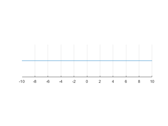
1.1.2 Non-negative numbers
In many economic problems, we have to restrict ourselves to numbers greater or equal to zero.
We can not consume from negative numbers of apples
We can not produce with negative labor and capital
We would be infinitely unhappy (die) if there is zero consumption in a year
We can use the following notation to define the set of non-negative real numbers:
\({R_{\ge 0} }\equiv \lbrace x\in R:x\ge 0\rbrace\), some authors use \({R_+ }\) instead of \({R_{\ge 0} }\)
And use inequality sign to define the set of real numbers greater than zero:
\({R_{>0} }\equiv \lbrace x\in R:x>0\rbrace\), some authors use \({R_{++} }\) instead of \({R_{>0} }\)
close all;
figure();
x = linspace(0,10);
line(x,0*ones(size(x)))
set(gca,'ytick',[],'Ycolor','w','box','off')
ylim([-0.1 0.1])
xlim([-10 10])
pbaspect([4 1 1])
grid on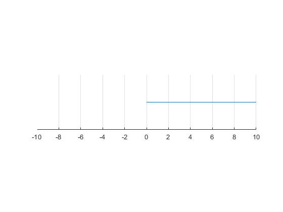
1.2 Interval Notations and Examples
Go back to fan’s MEconTools Package, Matlab Code Examples Repository (bookdown site), or Math for Econ with Matlab Repository (bookdown site).
When we look at the problem facing a household, we often have to restrict the choice set for example to an interval.
1.2.1 Closed Interval
For example, if \(x\) is hours working, perhaps the household has to work at least \(a\) hours and up to \(b\) hours, so his choice is between \(a\) and \(b\) hours inclusive.
The interval that is inclusive of both endpoints is called a closed interval (note the square brackets):
- closed interval: \(\left\lbrack a,b\right\rbrack \equiv \lbrace x\in R:a\le x\le b\rbrace\)
1.2.2 Open Interval
In general, an open interval is defined as (Note here we use parenthesis, not square brackest) :
- open interval:\(\left(a,b\right)\equiv \lbrace x\in R:a<x<b\rbrace\)
1.2.3 Half Open and Half Close Interval
We can also hafl half open intervals:
half open (half closed) interval: \(\left\lbrack a,b\right)\equiv \lbrace x\in R:a\le x<b\rbrace\)
half open (half closed) interval: \(\left(a,b\right\rbrack \equiv \lbrace x\in R:a<x\le b\rbrace\)
1.2.4 Graph
If you were to graph an interval, you can draw an empty circle at either end of an interval that is open, and a solid circle if it is closed at that end.
close all;
figure();
x = linspace(-1,5);
line(x,0*ones(size(x)))
set(gca,'ytick',[],'Ycolor','w','box','off')
ylim([-0.1 0.1])
xlim([-10  10])
pbaspect([4 1 1])
grid on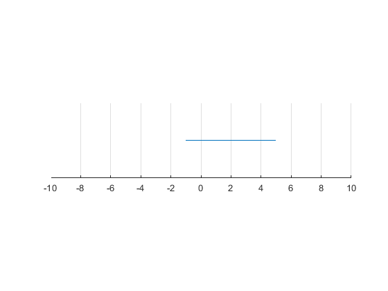
1.3 What is a Function?
Go back to fan’s MEconTools Package, Matlab Code Examples Repository (bookdown site), or Math for Econ with Matlab Repository (bookdown site).
function/mapping: a mapping (also called a function) is a rule that assigns to every element x of a set X a single element of a set Y. It is written as:
\[f:X\to Y\]
where the arrow indicates mapping, and the letter \(f\) symbolically specifies a rule of mapping. When we write:
\[y=f(x)\]
we are mapping from argument \(x\) in domain \(X\) to value \(y\) in co-domain Y.
Definitions:
domain: big \(X\) is the domain of \(f\)
argument: little \(x\) is an element in big \(X\), an argument of the function \(f\).
co-domain: big \(Y\) is the co-domain of \(f\).
image/value: when \(y=f(x)\), we refer to \(y\) as the image or value of \(x\) under \(f\).
range: \(f(X)=\lbrace y\in Y:y=f(x)\;\textrm{for}\;\textrm{some}\;x\in X\rbrace\)
graph: "The graph of a function of one variables consists of all points in the Cartesian plane whose coordinates (x,y) satisfy the equation y = f(x)" (SB)
In some textbooks, \(x\) is called independent or exogenous variables, and \(y\) is called dependent or endogenous variables. We will avoid using those words to avoid confusion.
This is a function:
figure();
x = 0:pi/100:2*pi;
y = sin(x);
plot(x,y);
grid on;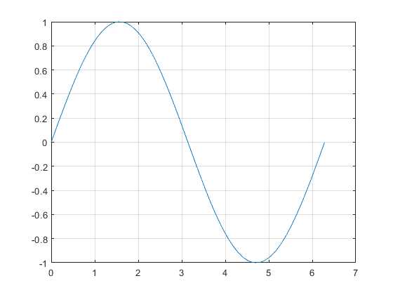
This is NOT a function:
figure();
x = 1; y=1; r=1;
th = 0:pi/50:2*pi;
xunit = r * cos(th) + x;
yunit = r * sin(th) + y;
h = plot(xunit, yunit);
grid on;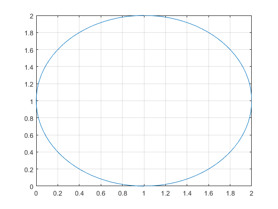
A Linear Function
A linear function, polynomial of degreee 1, has slope \(m\) and intercept \(b\). Linear functions have a constant slope.
figure();
m = 0.5;
b = 1;
ar_x = linspace(-5, 10, 100);
ar_y = ar_x*m + b;
h = plot(ar_x, ar_y);
% Title
title({['Linear function with slope m=' num2str(m) ' and y-intercept=' num2str(b)]});
% axis lines
xline0 = xline(0);
xline0.HandleVisibility = 'off';
yline0 = yline(0);
yline0.HandleVisibility = 'off';
grid on;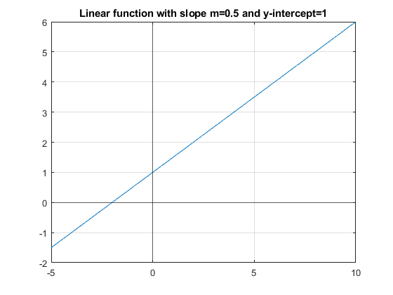
1.4 Function Notations
Go back to fan’s MEconTools Package, Matlab Code Examples Repository (bookdown site), or Math for Econ with Matlab Repository (bookdown site).
When you read your first economic papers, perhaps you are confused about function notation. Economic models include potentially a lot of variables, and different notations are used based on personal preference. Make sure you use consistent notations, and state clearly what your notations mean.
In general, the letter \(f\) represents a particular rule of mapping, if there are multiple functional relationships in an economic model, different letters could be used, for example:
\[y=Y(h),l=L(h),u=U(h)\]
These three equations could be from a model where:
\(h\) is the number of hours an individual works
\(y\) is the income that the individual makes as a function of work hours
\(l\) is the number of leisure hours remaining as a function work hours
\(u\) is the overall level of utility as a function of work hours.
Or you might potentially want to use superscripts:
\[y=f^y (h),l=f^l (h),u=f^w (h)\]
Or we could use the same letter (small cap) for function as the letter for the value of the function:
\[y=y(h),l=l(h),u=u(h)\]
Or maybe even more letters:
\[y=PROD(h),l=LEIS(h),u=UTIL(h)\]
Or perhaps different single letters than the output:
\[y=f(h),l=g(h),u=v(h)\]
Each notation structure could be confusing, make sure you are clear about what your notations mean. Math should help make our ideas more clear to ourselves and others, and that starts with clear functional notations.
1.5 Graphing Monomials and Polynomial of the 3rd Degree
Go back to fan’s MEconTools Package, Matlab Code Examples Repository (bookdown site), or Math for Econ with Matlab Repository (bookdown site).
1.5.1 Monomial
Functions of the form:
\[a\cdot x^k\]
are monomials.
\(a\) is any real number, it is the coefficient.
\(k\) is a positive integer, it is the degree of the monomial
1.5.2 Polynomial
Monomials added up together are polynomials
\[a+b\cdot x+c\cdot x^2 +d\cdot x^3 +e\cdot x^4\]
The coefficients \(a,b,c,d,e\) above could be positive or negative.
- Degree of Polynomial: We say that this polynomial has degree of 4. You find the largest degree monomial in the polynomial, and its degree is the degree of the whole polynomial.
1.5.3 Graphical Monomial Examples
Take a look at the function below, matlab makes it very easy to plot functions. You can see that when we shift the coefficient for the monomial, it rescales the function but does not change the ordinality.
Monomial when a = 0.75, a = 1, and a = 1.25:
clear all;
a = 0.75;
ffi_monomial_graph(a)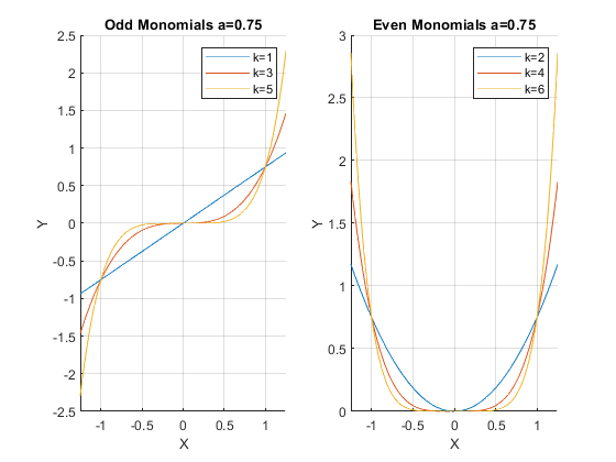
a = 1.25;
ffi_monomial_graph(a)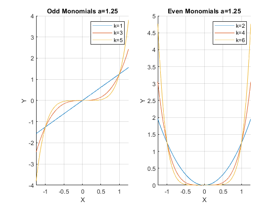
1.5.4 Polynomial of Degree Three
Some outcome is a function of a polynomial of degree three, what does this look like?
[fl_lower_bound, fl_uppper_bound] = deal(0.1, 0.9);
% Graph 1
[fl_constant, fl_lin, fl_quad, fl_cubic] = deal(0.131047762,0.002654614,-0.012944615,0.0086788);
ffi_poly3rd_degree(fl_lower_bound, fl_uppper_bound, fl_constant, fl_lin, fl_quad, fl_cubic);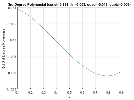
% Graph 2
[fl_constant, fl_lin, fl_quad, fl_cubic] = deal(1.406975108, -0.115556127, 0.343419845, -0.212016167);
ffi_poly3rd_degree(fl_lower_bound, fl_uppper_bound, fl_constant, fl_lin, fl_quad, fl_cubic);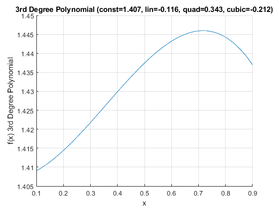
% Graph 3
[fl_constant, fl_lin, fl_quad, fl_cubic] = deal(1.102411416, -0.03056625, 0.146249875, -0.094270393);
ffi_poly3rd_degree(fl_lower_bound, fl_uppper_bound, fl_constant, fl_lin, fl_quad, fl_cubic);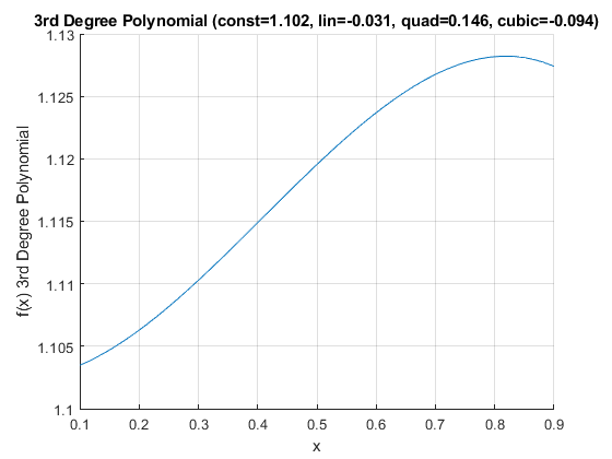
1.5.5 Mononomials Function
When we program, we can write functions, which have parameters
function ffi_monomial_graph(a)

% Define a symbolic monomial
syms x k
f(x, k) = a*x^k;

% Graph equation
close all;
figure();

%Subplot 1
subplot(1,2,1)
% Create minimum x and maximum x point where to draw the graph
x_lower_bd = -1.25;
x_upper_bd = +1.25;
% keep all figures, do not drop previous
hold on;
% Draw the function
ak1 = fplot(@(x) f(x, 1), [x_lower_bd, x_upper_bd]);
ak3 = fplot(@(x) f(x, 3), [x_lower_bd, x_upper_bd]);
ak5 = fplot(@(x) f(x, 5), [x_lower_bd, x_upper_bd]);
% Label
xlabel('X');
ylabel('Y');
xlim([x_lower_bd, x_upper_bd])
title(['Odd Monomials a=',num2str(a)])
legend('k=1','k=3', 'k=5');
grid on

% Subplot 2
subplot(1,2,2)
% Create minimum x and maximum x point where to draw the graph
x_lower_bd = -1.25;
x_upper_bd = +1.25;
% keep all figures, do not drop previous
hold on;
% Draw the function
ak2 = fplot(@(x) f(x, 2), [x_lower_bd, x_upper_bd]);
ak4 = fplot(@(x) f(x, 4), [x_lower_bd, x_upper_bd]);
ak6 = fplot(@(x) f(x, 6), [x_lower_bd, x_upper_bd]);
% Label
xlabel('X');
ylabel('Y');
xlim([x_lower_bd, x_upper_bd])
title(['Even Monomials a=', num2str(a)])
legend('k=2','k=4', 'k=6');
grid on
end
1.5.6 Polynomial of Degree Three Function
A function for graphing polynomial of the 3rd Degree.
function ffi_poly3rd_degree(fl_lower_bound, fl_uppper_bound, fl_constant, fl_lin, fl_quad, fl_cubic)

% Define a symbolic monomial
syms x
f(x) = fl_constant + fl_lin*x^2 + fl_quad*x^2 + fl_cubic*x^3;

% Graph equation
close all;
figure();

hold on;
% Draw the function
fplot(@(x) f(x), [fl_lower_bound, fl_uppper_bound]);
% Label
xlabel('x');
ylabel('f(x) 3rd Degree Polynomial');
xlim([fl_lower_bound, fl_uppper_bound])
% Title
ar_params = [fl_constant, fl_lin, fl_quad, fl_cubic];
ar_st_parms_names = ["const", "lin", "quad", "cubic"];
st_rounding = '.3f';
st_title_main = "3rd Degree Polynomial";
ar_st_params = strcat(ar_st_parms_names, compose(strcat("=%", st_rounding), ar_params));
st_param_pasted = strjoin(ar_st_params, ', ');
st_title_wth_params = strcat(st_title_main, ' (', st_param_pasted, ')');
title(st_title_wth_params);
grid on

end
1.6 Local and Global Maximum
Go back to fan’s MEconTools Package, Matlab Code Examples Repository (bookdown site), or Math for Econ with Matlab Repository (bookdown site).
Definition
Global Maximum: Function \(f\) defined on domain \(X\) has a global maximum at \(x^* \in X\) if for all \(x\in X\), \(f(x)\le f(x^* )\)
Local Maximum: Function \(f\) defined on domain \(X\) has a local maximum at \(x^* \in X\) if there exists an open interval \(\left(a,b\right)\), such that \(x^* \in \left(a,b\right)\), and for all \(x\in \left(a,b\right)\), \(f(x)\le f(x^* )\)
Many functions do not have maximum
We have utility function, production function, and budget constraints in economic models.
When households make choices, they are picking the bundle of goods that gives them the highest level of utility.
Most of the production and utility functions that we use do not have local or global maximum.
For example, a cobb-douglas production function will produce ever higher output with more labor and capital input.
And a log utility function will give higher utility with higher levels of consumption.
Note: When we combine perference and budget together, like we did in our two goods model, we could think about the optimal bundle of choices that achieves the highest level of utility given fixed budget in a household maximization problem.
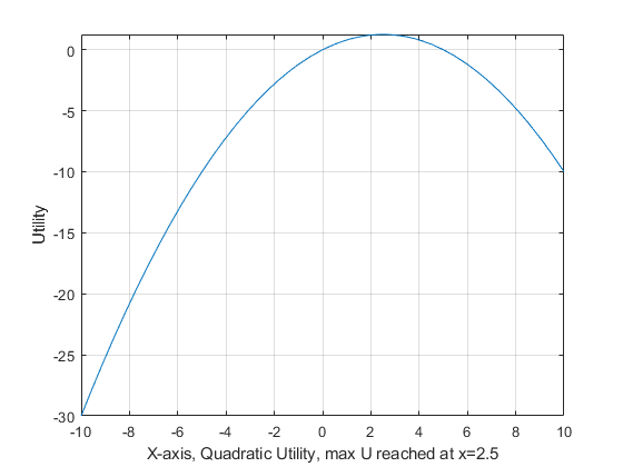
Quadratic Utility
A special utility function, quadratic utility, however, does have a single maximum.
\[U(x)=x-\alpha \cdot x^2\]
We can write down the equation using matlab’s symbolic package
% Parameter
a = 0.20;
% Create symbolic equation in matlab
syms x
f(x) = x - a*x^2
f(x) =
1em \(\displaystyle x-\frac{x^2 }{5}\)
Matlab Analytical Global Maximum for Quadratic Utility
Matlab can find the \(x\) value that maximizes the function by:
diff function: taking the derivative of f with respect to \(x\)
solve function: finding where the derivative crosses \(0\)
% Solve
maxofx = solve(diff(f, x), x)
maxofx =
1em \(\displaystyle \frac{5}{2}\)
% Convert symbolic to double precision
maxofx = double(maxofx)

maxofx = 2.5000
We have found the global maximum for the function.
A household will try to consume exactly this optimal amount of good if their budget allows.
With quadratic utility over one good, even if the household can afford to buy more goods than the maximum amount, they will not.
This could be used to approximate consumption of say how much rice a consumer wants for example.
Matlab Graphical Solution
% Graph equation
close all;
figure();
% Create minimum x and maximum x point where to draw the graph
x_lower_bd = min(-10, maxofx-abs(maxofx)/2);
x_upper_bd = max(10, maxofx+abs(maxofx)/2);
% Draw the function
fplot(f, [x_lower_bd, x_upper_bd]);
% Label
xlabel(['X-axis, Quadratic Utility, max U reached at x=', num2str(maxofx)])
ylabel(['Utility'])
grid on