A Choice Amongst Many--Household Borrowing in a Setting with Multiple Providers

• Robert M. Townsend
• Fan Wang

To demonstrate various aspects of the model and data, this is a work-in-progress website that provides links to various model code files and results for illustrative versions of the model. Most files on this page demonstrate model features in 2 or 3 period context. The full infinite horizon dynamic asset model with endogenous asset distributions for this model are shown in Section 5 and 6 of Fan’s Dynamic Asset Code Repository, where section 5 solves and simulates the model in an one dynamic asset environment, and section 6 solves the model in an environment with dynamic savings/borrowing as well as risky capital investment choices.

1. Introduction

We build a model in which households can use borrowing and savings jointly, and also use formal and informal borrowing options jointly. Most models of financial access do not distinguish between formal and informal options (For Example: Dabla-Norris, Ji, Townsend, and Unsal (2018)). Models that do distinguish formal and informal borrowing often do so in two period environments (For example: Karaivanov and Kessler (2018)) and rely on variations in fixed/transaction costs to justify the coexistence of formal and informal options (For Example: Gine (2011)).

Credit market options in the model here have three key features:

1. Formal borrowing choices come from a discrete choice set, informal borrowing with varying interest rates as well as savings help to complete the choice set.
2. Sometimes formal borrowing does not allow for roll-over (no-roll-over means new loans are issued only after the repayment of principles and interests). When this is the case, informal loans can act as bridge-loans to allow households to borrow again
3. When households are unable to repay debts, minimum consumption provides a consumption floor, and formal and informal debts are rolled forward, creating variations in repayment duration.

We find empirical evidence for these three model features in Thai Village Data, but these three model features have in general not been incorporated into models that study the co-existence of formal and informal credit markets.

We augment a standard dynamic heterogeneous agent model with exogenous incomplete borrowing, savings and investment choices with these three model features. We solve and estimate the model using data from Thailand.

2. Data Features

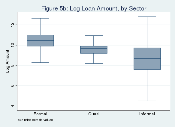
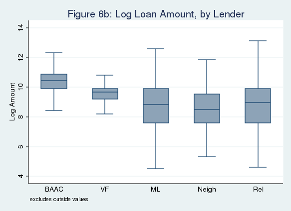
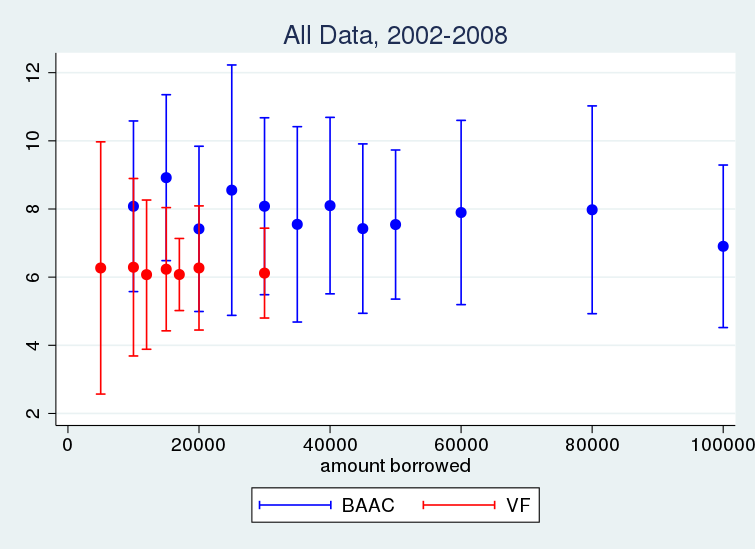
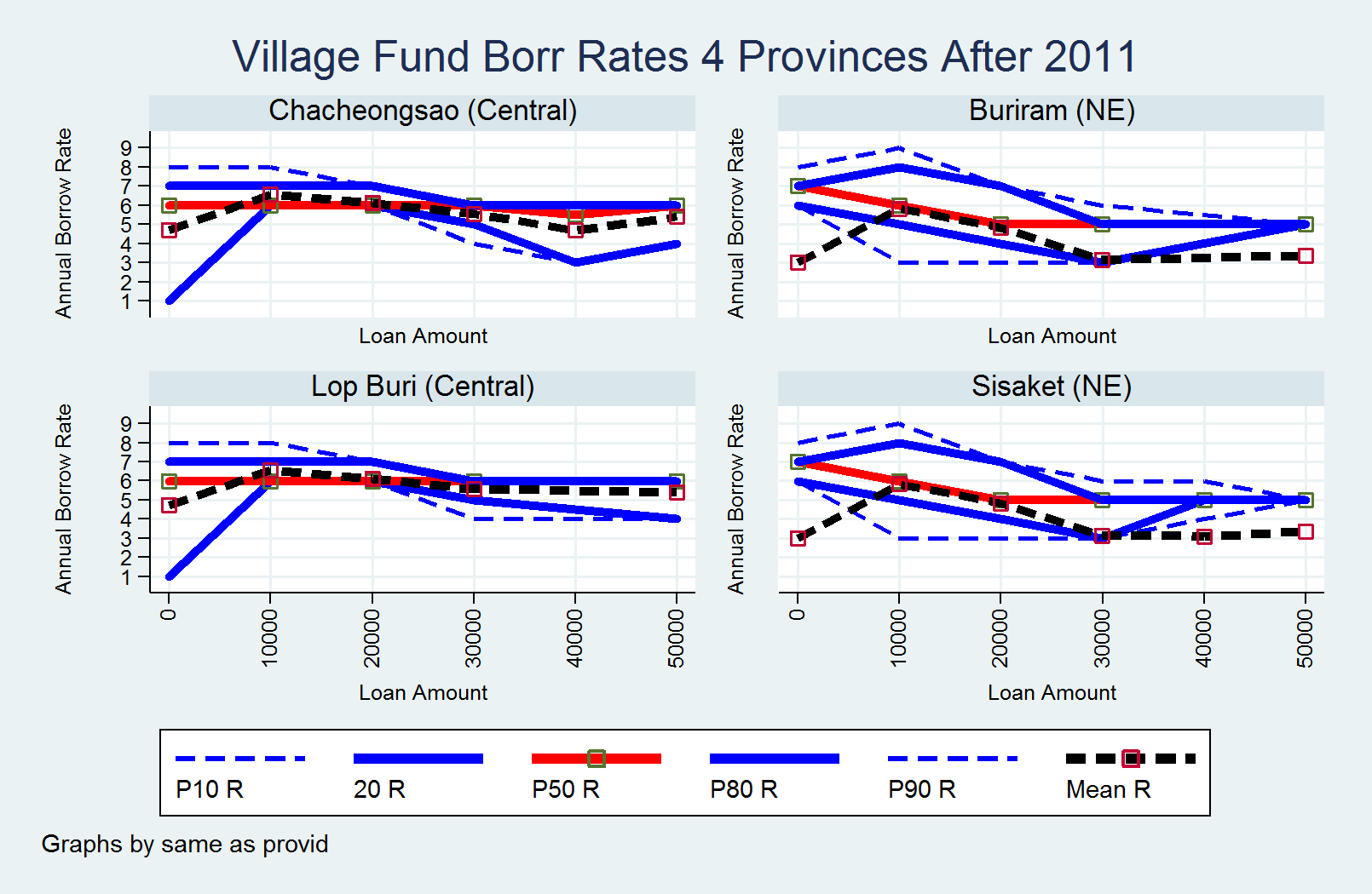
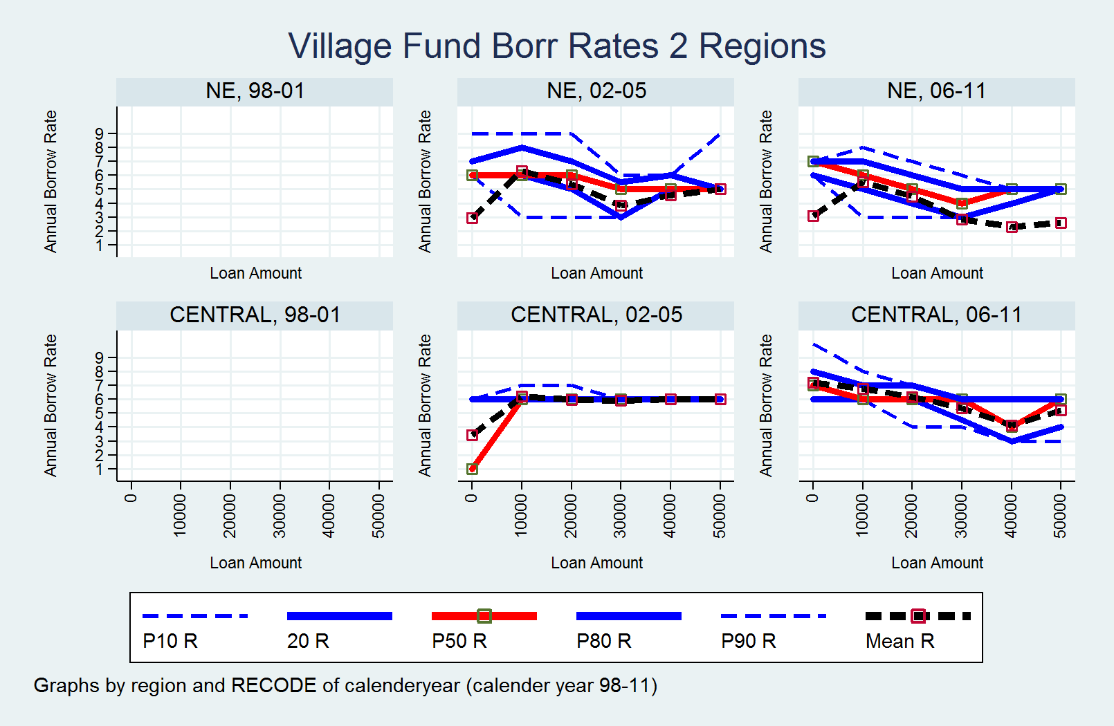
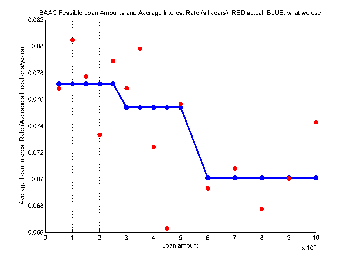
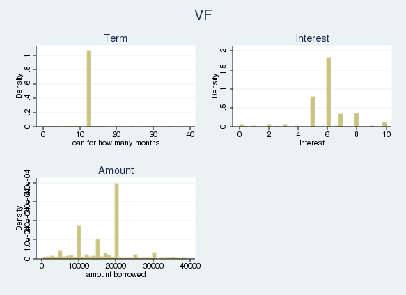
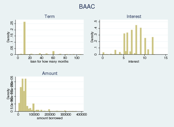
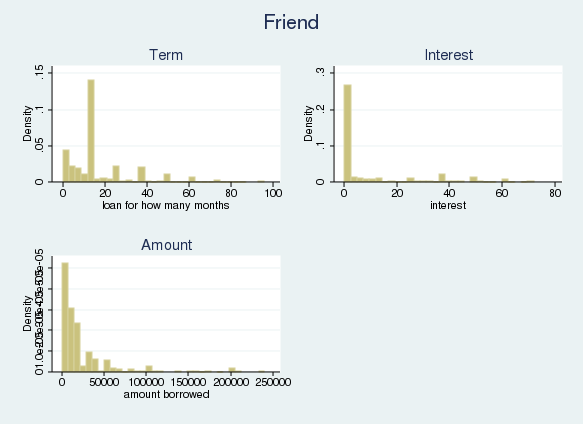
2.1 The Discretization of Formal Borrowing Choices

• Townsend Annual Data
  • Formal and Informal Group Statistics
    • Loan Size Distributions Formal and Informal
    • Loan Size Distributions Formal and Informal Subcategories
    • BAAC and VF Discrete Groupings and Interests
• Townsend Monthly Data
  • Rates Correlation
    • Interest Rate Correlation t and t+1 BAAC VF Informal
  • BAAC
    • VF Loan Size and Rates by Province
    • VF Loan Size and Rates by Years
    • BAAC Loan Size and Rates

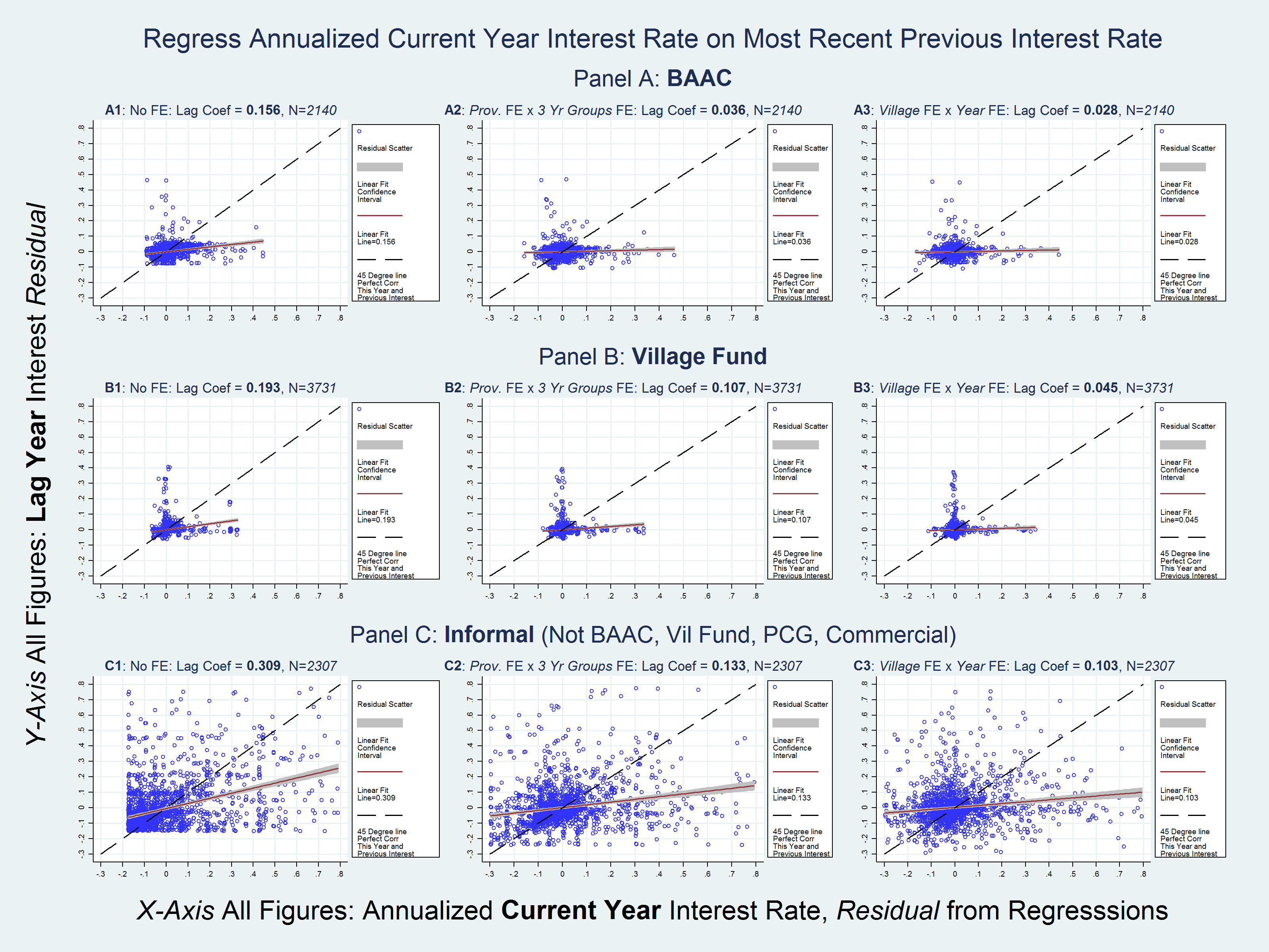
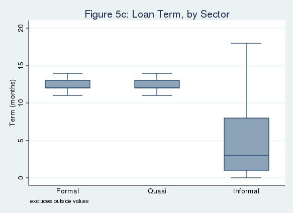
2.2 One-Period No-Roll-Over Formal Loans and Bridge Loan in the Data

• In the Thai Data, we observe significant amounts of bridge loans
  • Parit’s files we were looking at
• Specifically, traditionally, the BAAC required one year repayment of interest rates and principle before lending out new loans. Informal loans are often reported used as bridge loans to allow households to borrow from the informal sector in order to repay BAAC debt before borrowing from the BAAC again.
  • Formal and Informal Loan Lengths Box Plots
  • VF Loan Distribution
  • BAAC Loan Distribution
  • Informal Loans Distribution

3. Illustrating Key Model Components

Each of these three key model dimensions is defined and analyzed. Generally first in a two or three period model context without shocks, then in a model with shocks and with risky investments, and then in an infinite horizon context with endogenous asset. Along the steps, we calculate unconstrained optimal choices, the constrained optimal choices when only formal options are available (as: 1, discrete loan menu; 2, no-roll-over one-period loans), and the gains from the inclusion of informal options (as: 1, continuous informal loans with varying interest rates; 2, roll-over loans).

3.1 Limited Borrowing Choice Set

A standard formulation is that households can borrow from formal lenders, but there is a limit on borrowing. This constraint allows households to freely choose optimal borrowing quantity below the limit. This borrowing structure describes potentially a credit card.

In reality, in the context of development banking, borrowing could be limited to a menu of options: households face a finite discrete choice set of formal loans. This discreteness might arise because it is less costly for development banks to offer fewer borrowing options to small rural borrowers.

The discreteness of formal borrowing creates a need for using savings as well as informal borrowing to help complete the budget set.

By using 2-period models below, we clearly visualize changes in choice sets. The full dynamic models with uncertainty rely on the same underlying choice grid structures.

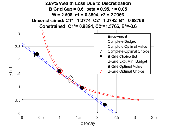
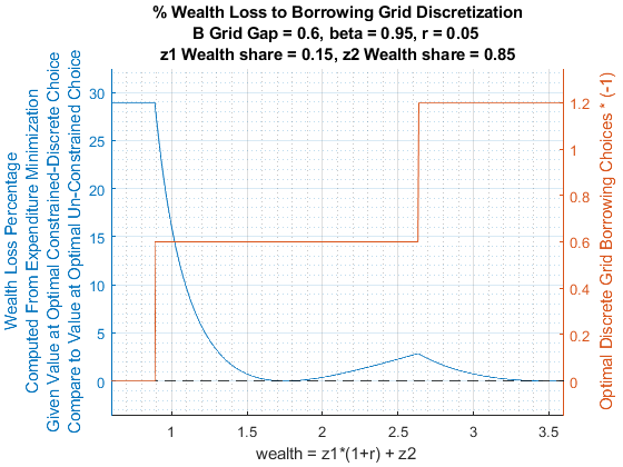
3.1.1 Borrowing Choice Set Discretization in a Deterministic Two Period Model

HTML | PDF | Matlab Livescript | Matlab M

• 2 Period Model.
• Standard borrowing constraint allows for any borrowing up to a limit.
• Here borrowing choices are restricted to a menu.

Summary Graph

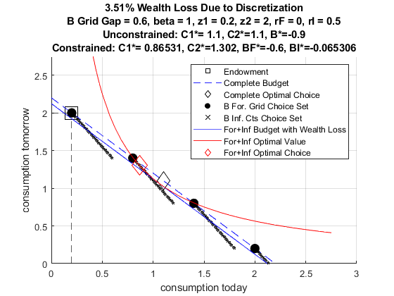
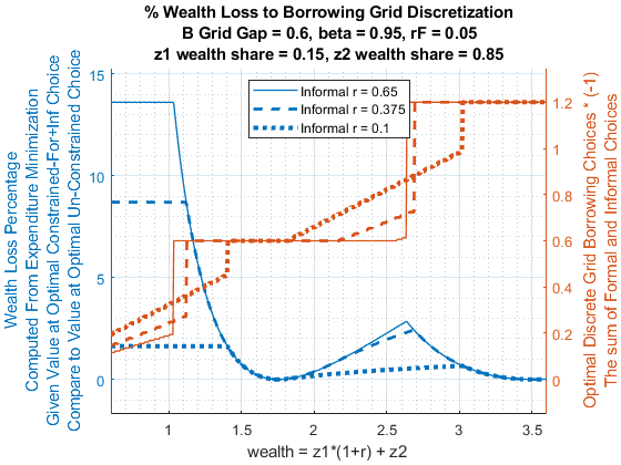
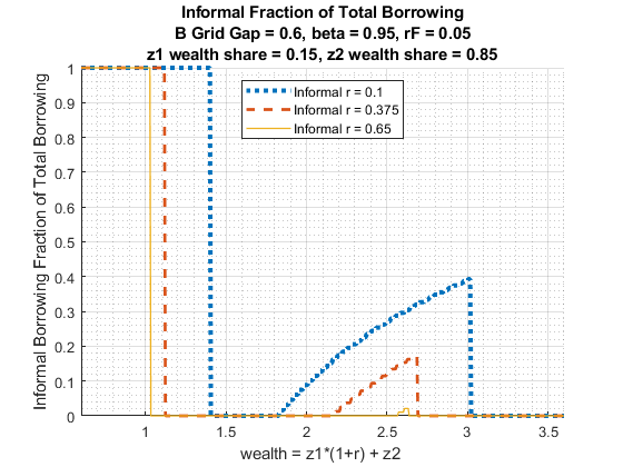
3.1.2 Informal Borrowing Partially Completes Formal Borrowing Frontier

HTML | PDF | Matlab Livescript | Matlab M

• 2 Period Model.
• Formal borrowing based on a menu of options.
• Informal borrowing at various interest rates partially completes the formal borrowing choice frontier.

Summary Graph

3.2 Bridge Loans

When do banks require the repayment of principles? Development financial institutions often offer one-year loans that require the repayment of interests as well as principles within a year.

Informal loans could be used as bridge loans. You borrow from informal lenders to repay the fraction of formal loan principal that you can not afford given your income realization.

In this section, borrowings are not restricted to a finite choice set as in the earlier section.

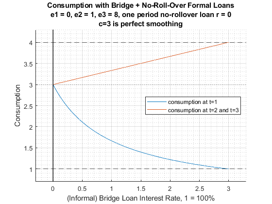
3.2.1 Multi-Period Loans, One-Period Loans, Roll-over Loans, Bridge Loans

HTML | PDF | Matlab Livescript | Matlab M

• Deterministic three period model.
• Define what are Multi-period, One-Period, Roll-over and Bridge Loans.
• Bridge loan helps to smooth consumption. Very high interest rate bridge loans can coexist with loan interest rate formal loans.

Summary Graph

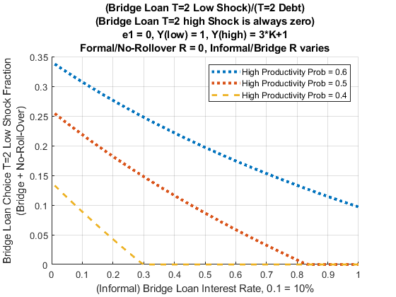
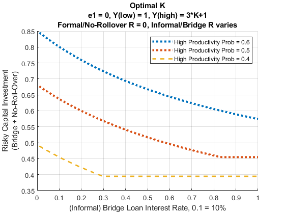
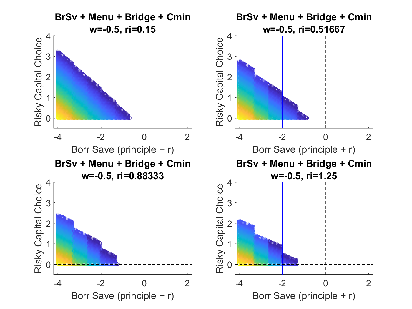
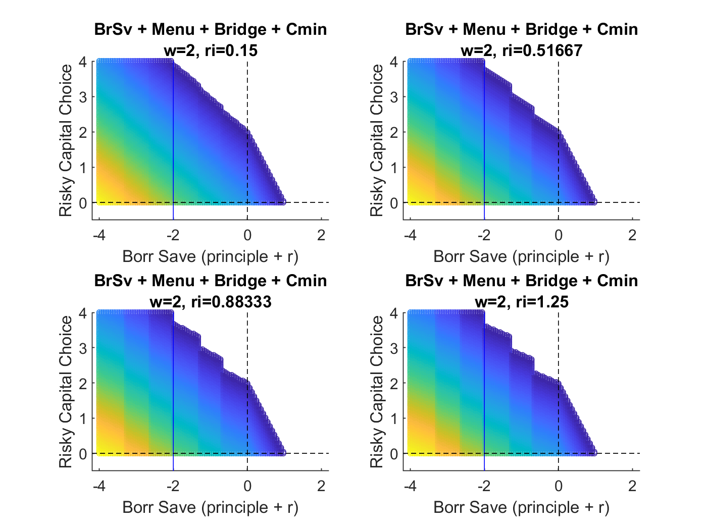
3.2.2 Bridge Loan, Uncertainty and Risky Investment

HTML | PDF | Matlab Livescript | Matlab M

• Three period model with shocks.
• Optimal risky investments, borrowing/savings and consumption with roll-over loans, and also with no-roll-over loans (requires principle repayment).
• Bridge loans help to repay existing debt.
• Very high interest rate (informal) bridge loan can co-exist with (formal) no-roll-over loans.
• Lower bridge loan interest rate, more borrowing and investments: high consumption in high productivity shock state, lower consumption along low productivity shock path (higher repayment needs).

Summary Graph

3.3 Debt and Default

We allow for default by incorporating a minimum consumption level. Minimum consumption breaks the natural borrowing constraint, and allows for significantly higher levels of borrowing and investments. Minimum consumption allows for the possibility of default. Here, we modify the default condition so that “default” means households will delay debt repayments until future periods: When household income (and bridge loan) are insufficient to repay debts owed, households pay as much as they can, resort to minimum consumption and continue repaying debts in future periods.

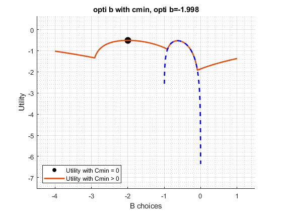
3.3.1 Minimum Consumption and Borrowing

HTML | PDF | Matlab Livescript | Matlab M

• Defining minimum consumption
• Minimum consumption enlarges choice sets

Summary Graph

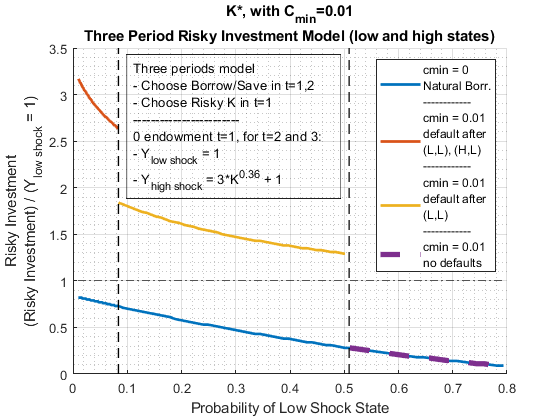
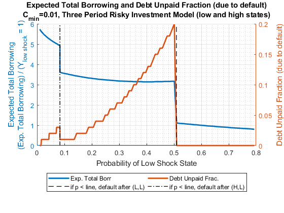
3.3.2 Minimum Consumption and Risky Investment

HTML | PDF | Matlab Livescript | Matlab M

• Minimum consumption with risky investments in a three period model
• Risky investment increases, borrowing increases, default now possible.

Summary Graph

4. Full Model

For our main model, model combines these three model features in a dynamic heterogeneous agent environment in which households make risky investment and safe asset choices. There are few models that consider both formal and informal borrowing choices in a dynamic context. In Banerjee, Breza, Duflo and Kinnan (2018), households can borrow from formal and informal options given two different borrowing bounds and interest rates. In Wang (2018), households can borrow and save formally and informally, but informal loans do not help to complete the budget set or act as bridge loans, and defaults are not allowed.

4.1 Choice Set

HTML | PDF | Matlab Livescript | Matlab M

• Features of model determine the choice set as well as credit costs.

4.2 Model Equations and Solution

Full model code and simulations are shown in 5 and 6 of Fan’s Dynamic Asset Code Repository, where section 5 solves and simulates the model in an one asset environment, and section 6 solves the model in an environment with savings as well as investment choices.

5. Estimation

5.1 Data for Estimation

PDF |

• Raw Data
• Building up interest rates variables
• Building up variables for formal and informal borrowing
• Building up savings variables
• Resulting monthly dataset combined with monthly household income and other balance sheet data
• Resulting annualized dataset