Chapter 2 Manipulate and Summarize Dataframes

2.1 Variables in Dataframes

2.1.1 Generate Dataframe

2.1.1.1 Simple Dataframe, Name Columns

# 5 by 3 matrix
mt_rnorm_a <- matrix(rnorm(4,mean=0,sd=1), nrow=5, ncol=3)

# Column Names
ar_st_varnames <- c('id','var1','varb','vartheta')

# Combine to tibble, add name col1, col2, etc.
tb_combine <- as_tibble(mt_rnorm_a) %>%
  rowid_to_column(var = "id") %>%
  rename_all(~c(ar_st_varnames))

# Display
kable(tb_combine) %>% kable_styling_fc()

id	var1	varb	vartheta
1	-1.1655448	-0.8185157	0.6849361
2	-0.8185157	0.6849361	-0.3200564
3	0.6849361	-0.3200564	-1.1655448
4	-0.3200564	-1.1655448	-0.8185157
5	-1.1655448	-0.8185157	0.6849361

2.1.1.2 Dataframe with Row and Column Names and Export

First, we generate an empty matrix. Second, we compute values to fill in matrix cells.

# an NA matrix
it_nrow <- 5
it_ncol <- 3
mt_na <- matrix(NA, nrow=it_nrow, ncol=it_ncol)

# array of nrow values
ar_it_nrow <- seq(1, it_nrow)
ar_it_ncol <- seq(1, it_ncol)

# Generate values in matrix
for (it_row in ar_it_nrow) {
  for (it_col in ar_it_ncol) {
    print(glue::glue("row={it_row} and col={it_col}"))
    mt_na[it_row, it_col] = it_row*it_col + it_row + it_col
  }
}

## row=1 and col=1
## row=1 and col=2
## row=1 and col=3
## row=2 and col=1
## row=2 and col=2
## row=2 and col=3
## row=3 and col=1
## row=3 and col=2
## row=3 and col=3
## row=4 and col=1
## row=4 and col=2
## row=4 and col=3
## row=5 and col=1
## row=5 and col=2
## row=5 and col=3

# Display
kable(mt_na) %>% kable_styling_fc()

3	5	7
5	8	11
7	11	15
9	14	19
11	17	23

Third, we label the rows and the columns. Note that we will include the column names as column names, but the row names will be included as a variable.

# Column Names
ar_st_col_names <- paste0('colval=', ar_it_ncol) 
ar_st_row_names <- paste0('rowval=', ar_it_nrow) 

# Create tibble, and add in column and row names
tb_row_col_named <- as_tibble(mt_na) %>%
  rename_all(~c(ar_st_col_names)) %>%
  mutate(row_name = ar_st_row_names) %>%
  select(row_name, everything())

# Display
kable(tb_row_col_named) %>% kable_styling_fc()

row_name	colval=1	colval=2	colval=3
rowval=1	3	5	7
rowval=2	5	8	11
rowval=3	7	11	15
rowval=4	9	14	19
rowval=5	11	17	23

Finally, we generate a file name for exporting this tibble to a CSV file. We create a file name with a time stamp.

# Create a file name with date stamp
st_datetime <- base::format(Sys.time(),  "%Y%m%d-%H%M%S")
# Copying a fixed date to avoid generating multiple testing files
# The date string below is generated by Sys.time()
st_snm_filename <- paste0("tibble_out_test_", st_datetime, '.csv')

# Create a file name with the time stamp. 
spn_file_path = file.path(
  "C:", "Users", "fan", 
  "R4Econ", "amto", "tibble", "_file",
  st_snm_filename,
  fsep = .Platform$file.sep)

# Save to file
write_csv(tb_row_col_named, spn_file_path)

2.1.1.3 Generate Tibble given Matrixes and Arrays

Given Arrays and Matrixes, Generate Tibble and Name Variables/Columns

naming tibble columns
tibble variable names
dplyr rename tibble
dplyr rename tibble all variables
dplyr rename all columns by index
dplyr tibble add index column
see also: SO-51205520

# Base Inputs
ar_col <- c(-1,+1)
mt_rnorm_a <- matrix(rnorm(4,mean=0,sd=1), nrow=2, ncol=2)
mt_rnorm_b <- matrix(rnorm(4,mean=0,sd=1), nrow=2, ncol=4)

# Combine Matrix
mt_combine <- cbind(ar_col, mt_rnorm_a, mt_rnorm_b)
colnames(mt_combine) <- c('ar_col',
                          paste0('matcolvar_grpa_', seq(1,dim(mt_rnorm_a)[2])),
                          paste0('matcolvar_grpb_', seq(1,dim(mt_rnorm_b)[2])))

# Variable Names
ar_st_varnames <- c('var_one',
                    paste0('tibcolvar_ga_', c(1,2)),
                    paste0('tibcolvar_gb_', c(1,2,3,4)))

# Combine to tibble, add name col1, col2, etc.
tb_combine <- as_tibble(mt_combine) %>% rename_all(~c(ar_st_varnames))

# Add an index column to the dataframe, ID column
tb_combine <- tb_combine %>% rowid_to_column(var = "ID")

# Change all gb variable names
tb_combine <- tb_combine %>%
                  rename_at(vars(starts_with("tibcolvar_gb_")),
                            funs(str_replace(., "_gb_", "_gbrenamed_")))

# Tibble back to matrix
mt_tb_combine_back <- data.matrix(tb_combine)

# Display
kable(mt_combine) %>% kable_styling_fc_wide()

ar_col	matcolvar_grpa_1	matcolvar_grpa_2	matcolvar_grpb_1	matcolvar_grpb_2	matcolvar_grpb_3	matcolvar_grpb_4
-1	-1.3115224	-0.1294107	-0.1513960	-3.2273228	-0.1513960	-3.2273228
1	-0.5996083	0.8867361	0.3297912	-0.7717918	0.3297912	-0.7717918

kable(tb_combine) %>% kable_styling_fc_wide()

ID	var_one	tibcolvar_ga_1	tibcolvar_ga_2	tibcolvar_gbrenamed_1	tibcolvar_gbrenamed_2	tibcolvar_gbrenamed_3	tibcolvar_gbrenamed_4
1	-1	-1.3115224	-0.1294107	-0.1513960	-3.2273228	-0.1513960	-3.2273228
2	1	-0.5996083	0.8867361	0.3297912	-0.7717918	0.3297912	-0.7717918

kable(mt_tb_combine_back) %>% kable_styling_fc_wide()

ID	var_one	tibcolvar_ga_1	tibcolvar_ga_2	tibcolvar_gbrenamed_1	tibcolvar_gbrenamed_2	tibcolvar_gbrenamed_3	tibcolvar_gbrenamed_4
1	-1	-1.3115224	-0.1294107	-0.1513960	-3.2273228	-0.1513960	-3.2273228
2	1	-0.5996083	0.8867361	0.3297912	-0.7717918	0.3297912	-0.7717918

2.1.1.4 Generate a Table from Lists

We run some function, whose outputs are named list, we store the values of the named list as additional rows into a dataframe whose column names are the names from named list.

First, we generate the function that returns named lists.

# Define a function
ffi_list_generator <- function(it_seed=123) {
  set.seed(it_seed)
  fl_abc <- rnorm(1)
  ar_efg <- rnorm(3)
  st_word <- sample(LETTERS, 5, replace = TRUE)
  ls_return <- list("abc" = fl_abc, "efg" = ar_efg, "opq" = st_word)
  return(ls_return)
}
# Run the function
it_seed=123
ls_return <- ffi_list_generator(it_seed) 
print(ls_return)

## $abc
## [1] -0.5604756
## 
## $efg
## [1] -0.23017749  1.55870831  0.07050839
## 
## $opq
## [1] "K" "E" "T" "N" "V"

Second, we list of lists by running the function above with different starting seeds. We store results in a two-dimensional list.

# Run function once to get length
ls_return_test <- ffi_list_generator(it_seed=123) 
it_list_len <- length(ls_return_test)

# list of list frame
it_list_of_list_len <- 5
ls_ls_return <- vector(mode = "list", length = it_list_of_list_len*it_list_len)
dim(ls_ls_return) <- c(it_list_of_list_len, it_list_len)

# Fill list of list
ar_seeds <- seq(123, 123 + it_list_of_list_len - 1)
it_ctr <- 0
for (it_seed in ar_seeds) {
  print(it_seed)
  it_ctr <- it_ctr + 1
  ls_return <- ffi_list_generator(it_seed) 
  ls_ls_return[it_ctr,] <- ls_return
}

## [1] 123
## [1] 124
## [1] 125
## [1] 126
## [1] 127

# print 2d list
print(ls_ls_return)

##      [,1]       [,2]      [,3]       
## [1,] -0.5604756 numeric,3 character,5
## [2,] -1.385071  numeric,3 character,5
## [3,] 0.933327   numeric,3 character,5
## [4,] 0.366734   numeric,3 character,5
## [5,] -0.5677337 numeric,3 character,5

Third, we convert the list to a tibble dataframe. Prior to conversion we add names to the 1st and 2nd dimensions of the list. Then we print the results.

# get names from named list
ar_st_names <- names(ls_return_test)
dimnames(ls_ls_return)[[2]] <- ar_st_names
dimnames(ls_ls_return)[[1]] <- paste0('seed_', ar_seeds)

# Convert to dataframe
tb_ls_ls_return <- as_tibble(ls_ls_return)

# print
kable(tb_ls_ls_return) %>% kable_styling_fc()

abc	efg	opq
-0.5604756	-0.23017749, 1.55870831, 0.07050839	K, E, T, N, V
-1.385071	0.03832318, -0.76303016, 0.21230614	J, A, O, T, N
0.933327	-0.52503178, 1.81443979, 0.08304562	C, T, M, S, K
0.366734	0.3964520, -0.7318437, 0.9462364	Z, L, J, Y, P
-0.5677337	-0.814760579, -0.493939596, 0.001818846	Y, C, O, F, U

Fourth, to export list to csv file, we need to unlist list contents. See also Create a tibble containing list columns

# Unlist 
tb_unlisted <- tb_ls_ls_return %>%
  rowwise() %>%
  mutate_if(is.list, 
    funs(paste(unlist(.), sep='', collapse=', ')))
# print on screen, can see values
print(tb_unlisted)

2.1.1.5 Rename Tibble with Numeric Column Names

After reshaping, often could end up with variable names that are all numeric, intgers for example, how to rename these variables to add a common prefix for example.

# Base Inputs
ar_col <- c(-1,+1)
mt_rnorm_c <- matrix(rnorm(4,mean=0,sd=1), nrow=5, ncol=10)
mt_combine <- cbind(ar_col, mt_rnorm_c)

# Variable Names
ar_it_cols_ctr <- seq(1, dim(mt_rnorm_c)[2])
ar_st_varnames <- c('var_one', ar_it_cols_ctr)

# Combine to tibble, add name col1, col2, etc.
tb_combine <- as_tibble(mt_combine) %>% rename_all(~c(ar_st_varnames))

# Add an index column to the dataframe, ID column
tb_combine_ori <- tb_combine %>% rowid_to_column(var = "ID")

# Change all gb variable names
tb_combine <- tb_combine_ori %>%
                  rename_at(
                    vars(num_range('',ar_it_cols_ctr)),
                    funs(paste0("rho", . , 'var'))
                    )

# Display
kable(tb_combine_ori) %>% kable_styling_fc_wide()

ID	var_one	1	2	3	4	5	6	7	8	9	10
1	-1	-0.1255472	0.5646199	0.1335086	-0.1059632	-0.1255472	0.5646199	0.1335086	-0.1059632	-0.1255472	0.5646199
2	1	0.5646199	0.1335086	-0.1059632	-0.1255472	0.5646199	0.1335086	-0.1059632	-0.1255472	0.5646199	0.1335086
3	-1	0.1335086	-0.1059632	-0.1255472	0.5646199	0.1335086	-0.1059632	-0.1255472	0.5646199	0.1335086	-0.1059632
4	1	-0.1059632	-0.1255472	0.5646199	0.1335086	-0.1059632	-0.1255472	0.5646199	0.1335086	-0.1059632	-0.1255472
5	-1	-0.1255472	0.5646199	0.1335086	-0.1059632	-0.1255472	0.5646199	0.1335086	-0.1059632	-0.1255472	0.5646199

kable(tb_combine) %>% kable_styling_fc_wide()

ID	var_one	rho1var	rho2var	rho3var	rho4var	rho5var	rho6var	rho7var	rho8var	rho9var	rho10var
1	-1	-0.1255472	0.5646199	0.1335086	-0.1059632	-0.1255472	0.5646199	0.1335086	-0.1059632	-0.1255472	0.5646199
2	1	0.5646199	0.1335086	-0.1059632	-0.1255472	0.5646199	0.1335086	-0.1059632	-0.1255472	0.5646199	0.1335086
3	-1	0.1335086	-0.1059632	-0.1255472	0.5646199	0.1335086	-0.1059632	-0.1255472	0.5646199	0.1335086	-0.1059632
4	1	-0.1059632	-0.1255472	0.5646199	0.1335086	-0.1059632	-0.1255472	0.5646199	0.1335086	-0.1059632	-0.1255472
5	-1	-0.1255472	0.5646199	0.1335086	-0.1059632	-0.1255472	0.5646199	0.1335086	-0.1059632	-0.1255472	0.5646199

2.1.1.6 Tibble Row and Column and Summarize

Show what is in the table: 1, column and row names; 2, contents inside table.

tb_iris <- as_tibble(iris)
print(rownames(tb_iris))

##   [1] "1"   "2"   "3"   "4"   "5"   "6"   "7"   "8"   "9"   "10"  "11"  "12"  "13" 
##  [14] "14"  "15"  "16"  "17"  "18"  "19"  "20"  "21"  "22"  "23"  "24"  "25"  "26" 
##  [27] "27"  "28"  "29"  "30"  "31"  "32"  "33"  "34"  "35"  "36"  "37"  "38"  "39" 
##  [40] "40"  "41"  "42"  "43"  "44"  "45"  "46"  "47"  "48"  "49"  "50"  "51"  "52" 
##  [53] "53"  "54"  "55"  "56"  "57"  "58"  "59"  "60"  "61"  "62"  "63"  "64"  "65" 
##  [66] "66"  "67"  "68"  "69"  "70"  "71"  "72"  "73"  "74"  "75"  "76"  "77"  "78" 
##  [79] "79"  "80"  "81"  "82"  "83"  "84"  "85"  "86"  "87"  "88"  "89"  "90"  "91" 
##  [92] "92"  "93"  "94"  "95"  "96"  "97"  "98"  "99"  "100" "101" "102" "103" "104"
## [105] "105" "106" "107" "108" "109" "110" "111" "112" "113" "114" "115" "116" "117"
## [118] "118" "119" "120" "121" "122" "123" "124" "125" "126" "127" "128" "129" "130"
## [131] "131" "132" "133" "134" "135" "136" "137" "138" "139" "140" "141" "142" "143"
## [144] "144" "145" "146" "147" "148" "149" "150"

colnames(tb_iris)

## [1] "Sepal.Length" "Sepal.Width"  "Petal.Length" "Petal.Width"  "Species"

colnames(tb_iris)

## [1] "Sepal.Length" "Sepal.Width"  "Petal.Length" "Petal.Width"  "Species"

summary(tb_iris)

##   Sepal.Length    Sepal.Width     Petal.Length    Petal.Width          Species  
##  Min.   :4.300   Min.   :2.000   Min.   :1.000   Min.   :0.100   setosa    :50  
##  1st Qu.:5.100   1st Qu.:2.800   1st Qu.:1.600   1st Qu.:0.300   versicolor:50  
##  Median :5.800   Median :3.000   Median :4.350   Median :1.300   virginica :50  
##  Mean   :5.843   Mean   :3.057   Mean   :3.758   Mean   :1.199                  
##  3rd Qu.:6.400   3rd Qu.:3.300   3rd Qu.:5.100   3rd Qu.:1.800                  
##  Max.   :7.900   Max.   :4.400   Max.   :6.900   Max.   :2.500

2.1.1.7 Sorting and Rank

2.1.1.7.1 Sorting

dplyr arrange desc reverse
dplyr sort

# Sort in Ascending Order
tb_iris %>% select(Species, Sepal.Length, everything()) %>%
  arrange(Species, Sepal.Length) %>% head(10) %>%
  kable() %>% kable_styling_fc()

Species	Sepal.Length	Sepal.Width	Petal.Length	Petal.Width
setosa	4.3	3.0	1.1	0.1
setosa	4.4	2.9	1.4	0.2
setosa	4.4	3.0	1.3	0.2
setosa	4.4	3.2	1.3	0.2
setosa	4.5	2.3	1.3	0.3
setosa	4.6	3.1	1.5	0.2
setosa	4.6	3.4	1.4	0.3
setosa	4.6	3.6	1.0	0.2
setosa	4.6	3.2	1.4	0.2
setosa	4.7	3.2	1.3	0.2

# Sort in Descending Order
tb_iris %>% select(Species, Sepal.Length, everything()) %>%
  arrange(desc(Species), desc(Sepal.Length)) %>% head(10) %>%
  kable() %>% kable_styling_fc()

Species	Sepal.Length	Sepal.Width	Petal.Length	Petal.Width
virginica	7.9	3.8	6.4	2.0
virginica	7.7	3.8	6.7	2.2
virginica	7.7	2.6	6.9	2.3
virginica	7.7	2.8	6.7	2.0
virginica	7.7	3.0	6.1	2.3
virginica	7.6	3.0	6.6	2.1
virginica	7.4	2.8	6.1	1.9
virginica	7.3	2.9	6.3	1.8
virginica	7.2	3.6	6.1	2.5
virginica	7.2	3.2	6.0	1.8

2.1.1.7.2 Create a Ranking Variable

We use dplyr’s ranking functions to generate different types of ranking variables.

The example below demonstrates the differences between the functions row_number(), min_rank(), and dense_rank().

row_number: Given 10 observations, generates index from 1 to 10, ties are given different ranks.
min_rank: Given 10 observations, generates rank where second-rank ties are both given “silver”, and the 4th highest ranked variable not given medal.
dense_rank: Given 10 observations, generates rank where second-rank ties are both given “silver” (2nd rank), and the 4th highest ranked variable is given “bronze” (3rd rank), there are no gaps between ranks.

Note that we have “desc(var_name)” in order to generate the variable based on descending sort of the the “var_name” variable.

tb_iris %>%
  select(Species, Sepal.Length) %>% head(10) %>%
  mutate(row_number = row_number(desc(Sepal.Length)),
         min_rank = min_rank(desc(Sepal.Length)),
         dense_rank = dense_rank(desc(Sepal.Length))) %>%
  kable(caption = "Ranking variable") %>% kable_styling_fc()

Table 2.1: Ranking variable
Species	Sepal.Length	row_number	min_rank	dense_rank
setosa	5.1	2	2	2
setosa	4.9	5	5	4
setosa	4.7	7	7	5
setosa	4.6	8	8	6
setosa	5.0	3	3	3
setosa	5.4	1	1	1
setosa	4.6	9	8	6
setosa	5.0	4	3	3
setosa	4.4	10	10	7
setosa	4.9	6	5	4

2.1.1.8 REconTools Summarize over Tible

Use R4Econ’s summary tool.

df_summ_stats <- REconTools::ff_summ_percentiles(tb_iris)
kable(t(df_summ_stats)) %>% kable_styling_fc_wide()

stats	n	unique	NAobs	ZEROobs	mean	sd	cv	min	p01	p05	p10	p25	p50	p75	p90	p95	p99	max
Petal.Length	150	43	0	0	3.758000	1.7652982	0.4697441	1.0	1.149	1.300	1.4	1.6	4.35	5.1	5.80	6.100	6.700	6.9
Petal.Width	150	22	0	0	1.199333	0.7622377	0.6355511	0.1	0.100	0.200	0.2	0.3	1.30	1.8	2.20	2.300	2.500	2.5
Sepal.Length	150	35	0	0	5.843333	0.8280661	0.1417113	4.3	4.400	4.600	4.8	5.1	5.80	6.4	6.90	7.255	7.700	7.9
Sepal.Width	150	23	0	0	3.057333	0.4358663	0.1425642	2.0	2.200	2.345	2.5	2.8	3.00	3.3	3.61	3.800	4.151	4.4

2.1.2 Generate Categorical Variables

2.1.2.1 Cut Continuous Variable to Categorical Variable

We have a continuous variable, we cut it with explicitly specified cuts to generate a categorical variable, and label it. We will use base::cut().

# break points to specific
fl_min_mpg <- min(mtcars$mpg)
fl_max_mpg <- max(mtcars$mpg)
ar_fl_cuts <- c(10, 20, 30, 40)
# generate labels
ar_st_cuts_lab <- c("10<=mpg<20", "20<=mpg<30", "30<=mpg<40")
# generate new variable
mtcars_cate <- mtcars %>% 
  tibble::rownames_to_column(var = "cars") %>%
  mutate(mpg_grp = base::cut(mpg,
      breaks = ar_fl_cuts, 
      labels = ar_st_cuts_lab,
      # if right is FALSE, interval is closed on the left
      right = FALSE
    )
  ) %>% select(cars, mpg_grp, mpg) %>% 
  arrange(mpg) %>% group_by(mpg_grp) %>%
  slice_head(n=3)
# Display
st_caption <- "Cuts a continuous var to a categorical var with labels"
kable(mtcars_cate,
    caption = st_caption
) %>% kable_styling_fc()

Table 2.2: Cuts a continuous var to a categorical var with labels
cars	mpg_grp	mpg
Cadillac Fleetwood	10<=mpg<20	10.4
Lincoln Continental	10<=mpg<20	10.4
Camaro Z28	10<=mpg<20	13.3
Mazda RX4	20<=mpg<30	21.0
Mazda RX4 Wag	20<=mpg<30	21.0
Hornet 4 Drive	20<=mpg<30	21.4
Honda Civic	30<=mpg<40	30.4
Lotus Europa	30<=mpg<40	30.4
Fiat 128	30<=mpg<40	32.4

2.1.2.2 Factor, Label, Cross and Graph

Generate a Scatter plot with different colors representing different categories. There are multiple underlying factor/categorical variables, for example two binary variables. Generate scatter plot with colors for the combinations of these two binary variables.

We combine here the vs and am variables from the mtcars dataset. vs is engine shape, am is auto or manual shift. We will generate a scatter plot of mpg and qsec over four categories with different colors.

am: Transmission (0 = automatic, 1 = manual)
vs: Engine (0 = V-shaped, 1 = straight)
mpg: miles per galon
qsec: 1/4 mile time

# First make sure these are factors
tb_mtcars <- as_tibble(mtcars) %>% 
  mutate(vs = as_factor(vs), am = as_factor(am))

# Second Label the Factors
am_levels <- c(auto_shift = "0", manual_shift = "1")
vs_levels <- c(vshaped_engine = "0", straight_engine = "1")
tb_mtcars <- tb_mtcars %>% 
  mutate(vs = fct_recode(vs, !!!vs_levels),
         am = fct_recode(am, !!!am_levels))

# Third Combine Factors
tb_mtcars_selected <- tb_mtcars %>%
  mutate(vs_am = fct_cross(vs, am, sep='_', keep_empty = FALSE)) %>%
  select(mpg, qsec, vs_am)

# relabel interaction variables
am_vs_levels <- c("vshape (engine) and auto (shift)" = "vshaped_engine_auto_shift", 
                  "vshape (engine) and manual (shift)" = "vshaped_engine_manual_shift", 
                  "straight (engine) and auto (shift)" = "straight_engine_auto_shift", 
                  "straight (engine) and manual (shift)" = "straight_engine_manual_shift")
tb_mtcars_selected <- tb_mtcars_selected %>%
  mutate(vs_am = fct_recode(vs_am, !!!am_vs_levels))

# Show
print(tb_mtcars_selected[1:10,])

Now we generate scatter plot based on the combined factors

# Labeling
st_title <- paste0('Distribution of MPG and QSEC from mtcars')
st_subtitle <- paste0('https://fanwangecon.github.io/',
                      'R4Econ/amto/tibble/htmlpdfr/fs_tib_factors.html')
st_caption <- paste0('mtcars dataset, ',
                     'https://fanwangecon.github.io/R4Econ/')
st_x_label <- 'MPG = Miles per Gallon'
st_y_label <- 'QSEC = time for 1/4 Miles'

# Graphing
plt_mtcars_scatter <- 
  ggplot(tb_mtcars_selected, 
         aes(x=mpg, y=qsec, colour=vs_am, shape=vs_am)) +
  geom_jitter(size=3, width = 0.15) +
  labs(title = st_title, subtitle = st_subtitle,
       x = st_x_label, y = st_y_label, caption = st_caption) +
  theme_bw()

# show
print(plt_mtcars_scatter)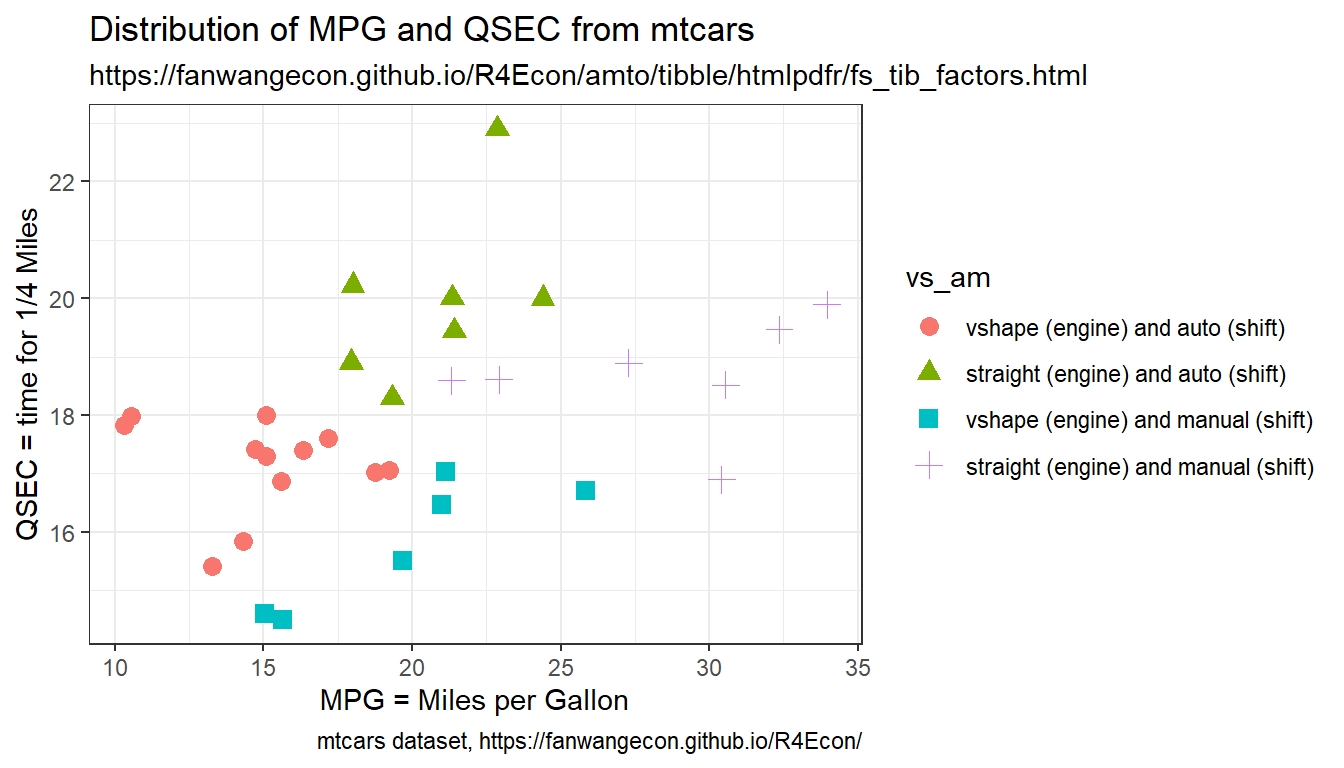

2.1.3 Drawly Random Rows

2.1.3.1 Draw Random Subset of Sample

r random discrete

We have a sample of N individuals in some dataframe. Draw without replacement a subset \(M<N\) of rows.

# parameters, it_M < it_N
it_N <- 10
it_M <- 5

# Draw it_m from indexed list of it_N
set.seed(123)
ar_it_rand_idx <- sample(it_N, it_M, replace=FALSE)

# dataframe
df_full <- as_tibble(matrix(rnorm(4,mean=0,sd=1), nrow=it_N, ncol=4)) %>% rowid_to_column(var = "ID")

# random Subset
df_rand_sub_a <- df_full[ar_it_rand_idx,]

# Random subset also
df_rand_sub_b <- df_full[sample(dim(df_full)[1], it_M, replace=FALSE),]

# Print
# Display
kable(df_full) %>% kable_styling_fc()

ID	V1	V2	V3	V4
1	0.1292877	0.4609162	0.1292877	0.4609162
2	1.7150650	-1.2650612	1.7150650	-1.2650612
3	0.4609162	0.1292877	0.4609162	0.1292877
4	-1.2650612	1.7150650	-1.2650612	1.7150650
5	0.1292877	0.4609162	0.1292877	0.4609162
6	1.7150650	-1.2650612	1.7150650	-1.2650612
7	0.4609162	0.1292877	0.4609162	0.1292877
8	-1.2650612	1.7150650	-1.2650612	1.7150650
9	0.1292877	0.4609162	0.1292877	0.4609162
10	1.7150650	-1.2650612	1.7150650	-1.2650612

kable(df_rand_sub_a) %>% kable_styling_fc()

ID	V1	V2	V3	V4
3	0.4609162	0.1292877	0.4609162	0.1292877
10	1.7150650	-1.2650612	1.7150650	-1.2650612
2	1.7150650	-1.2650612	1.7150650	-1.2650612
8	-1.2650612	1.7150650	-1.2650612	1.7150650
6	1.7150650	-1.2650612	1.7150650	-1.2650612

kable(df_rand_sub_b) %>% kable_styling_fc()

ID	V1	V2	V3	V4
5	0.1292877	0.4609162	0.1292877	0.4609162
3	0.4609162	0.1292877	0.4609162	0.1292877
9	0.1292877	0.4609162	0.1292877	0.4609162
1	0.1292877	0.4609162	0.1292877	0.4609162
4	-1.2650612	1.7150650	-1.2650612	1.7150650

2.1.3.2 Random Subset of Panel

There are \(N\) individuals, each could be observed \(M\) times, but then select a subset of rows only, so each person is randomly observed only a subset of times. Specifically, there there are 3 unique students with student ids, and the second variable shows the random dates in which the student showed up in class, out of the 10 classes available.

# Define
it_N <- 3
it_M <- 10
svr_id <- 'student_id'

# dataframe
set.seed(123)
df_panel_rand <- as_tibble(matrix(it_M, nrow=it_N, ncol=1)) %>%
  rowid_to_column(var = svr_id) %>%
  uncount(V1) %>%
  group_by(!!sym(svr_id)) %>% mutate(date = row_number()) %>%
  ungroup() %>% mutate(in_class = case_when(rnorm(n(),mean=0,sd=1) < 0 ~ 1, TRUE ~ 0)) %>%
  dplyr::filter(in_class == 1) %>% select(!!sym(svr_id), date) %>%
  rename(date_in_class = date)

# Print
kable(df_panel_rand) %>% kable_styling_fc()

student_id	date_in_class
1	1
1	2
1	8
1	9
1	10
2	5
2	8
2	10
3	1
3	2
3	3
3	4
3	5
3	6
3	9

2.1.4 Generate Variables Conditional On Others

2.1.4.1 Categorical Variable based on Several Variables

Given several other variables, and generate a new variable when these varaibles satisfy conditions. Note that case_when are ifelse type statements. So below

group one is below 16 MPG
when do qsec >= 20 second line that is elseif, only those that are >=16 are considered here
then think about two dimensional mpg and qsec grid, the lower-right area, give another category to manual cars in that group

First, we generate categorical variables based on the characteristics of several variables.

# Get mtcars
df_mtcars <- mtcars

# case_when with mtcars
df_mtcars <- df_mtcars %>%
    mutate(
        mpg_qsec_am_grp =
            case_when(
                mpg < 16 ~ "< 16 MPG",
                qsec >= 20 ~ "> 16 MPG & qsec >= 20",
                am == 1 ~ "> 16 MPG & asec < 20 & manual",
                TRUE ~ "Others"
            )
    )

Now we generate scatter plot based on the combined factors

# Labeling
st_title <- paste0("Use case_when To Generate ifelse Groupings")
st_subtitle <- paste0(
    "https://fanwangecon.github.io/",
    "R4Econ/amto/tibble/htmlpdfr/fs_tib_na.html"
)
st_caption <- paste0(
    "mtcars dataset, ",
    "https://fanwangecon.github.io/R4Econ/"
)
st_x_label <- "MPG = Miles per Gallon"
st_y_label <- "QSEC = time for 1/4 Miles"

# Graphing
plt_mtcars_casewhen_scatter <-
    ggplot(
        df_mtcars,
        aes(
            x = mpg, y = qsec,
            colour = mpg_qsec_am_grp,
            shape = mpg_qsec_am_grp
        )
    ) +
    geom_jitter(size = 3, width = 0.15) +
    labs(
        title = st_title, subtitle = st_subtitle,
        x = st_x_label, y = st_y_label, caption = st_caption
    ) +
    theme_bw()

# show
print(plt_mtcars_casewhen_scatter)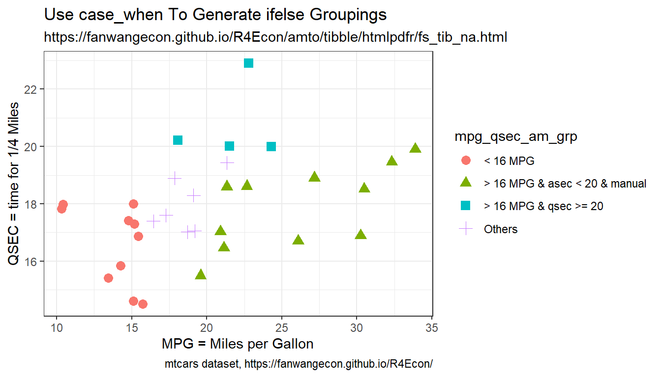

2.1.4.2 Categorical Variables based on one Continuous Variable

We generate one categorical variable for gear, based on “continuous” gear values. Note that the same categorical label appears for gear is 3 as well as gear is 5.

# Generate a categorical variable
df_mtcars <- df_mtcars %>%
    mutate(gear_cate = case_when(
        gear == 3 ~ "gear is 3",
        gear == 4 ~ "gear is 4",
        gear == 5 & hp <= 110 ~ "gear 5 hp les sequal 110",
        gear == 5 & hp > 110 & hp <= 200 ~ "gear 5 hp 110 to 130",
        TRUE ~ "otherwise"
    ))
# Tabulate
df_mtcars_gear_tb <- df_mtcars %>% 
  group_by(gear_cate, gear) %>%
  tally() %>%
  spread(gear_cate, n)
# Display
st_title <- "Categorical from continuous with non-continuous values matching to same key"
df_mtcars_gear_tb %>% kable(caption = st_title) %>%
  kable_styling_fc()

Table 2.3: Categorical from continuous with non-continuous values matching to same key
gear	gear 5 hp 110 to 130	gear 5 hp les sequal 110	gear is 3	gear is 4	otherwise
3	NA	NA	15	NA	NA
4	NA	NA	NA	12	NA
5	2	1	NA	NA	2

2.1.4.3 Generate NA values if Variables have Certain Value

In the example below, in one line:

generate a random standard normal vector
two set na methods:
- if the value of the standard normal is negative, set value to -999, otherwise MPG, replace the value -999 with NA
- case_when only with type specific NA values
- Assigning NA yields error in case_when
- note we need to conform NA to type
generate new categorical variable based on NA condition using is.na with both string and numeric NAs jointly considered.
- fake NA string to be printed on chart

# Get mtcars
df_mtcars <- mtcars

# Make some values of mpg randomly NA
# the NA has to conform to the type of the remaining values for the new variable
# NA_real_, NA_character_, NA_integer_, NA_complex_
set.seed(2341)
df_mtcars <- df_mtcars %>%
    mutate(mpg_wth_NA1 = na_if(
        case_when(
            rnorm(n(), mean = 0, sd = 1) < 0 ~ -999,
            TRUE ~ mpg
        ),
        -999
    )) %>%
    mutate(mpg_wth_NA2 = case_when(
        rnorm(n(), mean = 0, sd = 1) < 0 ~ NA_real_,
        TRUE ~ mpg
    )) %>%
    mutate(mpg_wth_NA3 = case_when(
        rnorm(n(), mean = 0, sd = 1) < 0 ~ NA_character_,
        TRUE ~ "shock > 0 string"
    ))

# Generate New Variables based on if mpg_wth_NA is NA or not
# same variable as above, but now first a category based on if NA
# And we generate a fake string "NA" variable, this is not NA
# the String NA allows for it to be printed on figure
df_mtcars <- df_mtcars %>%
    mutate(
        group_with_na =
            case_when(
                is.na(mpg_wth_NA2) & is.na(mpg_wth_NA3) ~
                    "Rand String and Rand Numeric both NA",
                mpg < 16 ~ "< 16 MPG",
                qsec >= 20 ~ "> 16 MPG & qsec >= 20",
                am == 1 ~ "> 16 MPG & asec < 20 & manual",
                TRUE ~ "Fake String NA"
            )
    )

# show
kable(head(df_mtcars %>% select(starts_with("mpg")), 13)) %>%
    kable_styling_fc()

	mpg	mpg_wth_NA1	mpg_wth_NA2	mpg_wth_NA3
Mazda RX4	21.0	NA	NA	shock > 0 string
Mazda RX4 Wag	21.0	21.0	21.0	NA
Datsun 710	22.8	NA	NA	NA
Hornet 4 Drive	21.4	NA	21.4	NA
Hornet Sportabout	18.7	NA	18.7	NA
Valiant	18.1	18.1	NA	shock > 0 string
Duster 360	14.3	14.3	NA	shock > 0 string
Merc 240D	24.4	NA	24.4	NA
Merc 230	22.8	22.8	22.8	NA
Merc 280	19.2	19.2	NA	NA
Merc 280C	17.8	NA	NA	NA
Merc 450SE	16.4	16.4	16.4	NA
Merc 450SL	17.3	NA	NA	shock > 0 string

# # Setting to NA
# df.reg.use <- df.reg.guat %>% filter(!!sym(var.mth) != 0)
# df.reg.use.log <- df.reg.use
# df.reg.use.log[which(is.nan(df.reg.use$prot.imputed.log)),] = NA
# df.reg.use.log[which(df.reg.use$prot.imputed.log==Inf),] = NA
# df.reg.use.log[which(df.reg.use$prot.imputed.log==-Inf),] = NA
# df.reg.use.log <- df.reg.use.log %>% drop_na(prot.imputed.log)
# # df.reg.use.log$prot.imputed.log

Now we generate scatter plot based on the combined factors, but now with the NA category

# Labeling
st_title <- paste0(
    "Use na_if and is.na to Generate and Distinguish NA Values\n",
    "NA_real_, NA_character_, NA_integer_, NA_complex_"
)
st_subtitle <- paste0(
    "https://fanwangecon.github.io/",
    "R4Econ/amto/tibble/htmlpdfr/fs_tib_na.html"
)
st_caption <- paste0(
    "mtcars dataset, ",
    "https://fanwangecon.github.io/R4Econ/"
)
st_x_label <- "MPG = Miles per Gallon"
st_y_label <- "QSEC = time for 1/4 Miles"

# Graphing
plt_mtcars_ifisna_scatter <-
    ggplot(
        df_mtcars,
        aes(
            x = mpg, y = qsec,
            colour = group_with_na,
            shape = group_with_na
        )
    ) +
    geom_jitter(size = 3, width = 0.15) +
    labs(
        title = st_title, subtitle = st_subtitle,
        x = st_x_label, y = st_y_label, caption = st_caption
    ) +
    theme_bw()

# show
print(plt_mtcars_ifisna_scatter)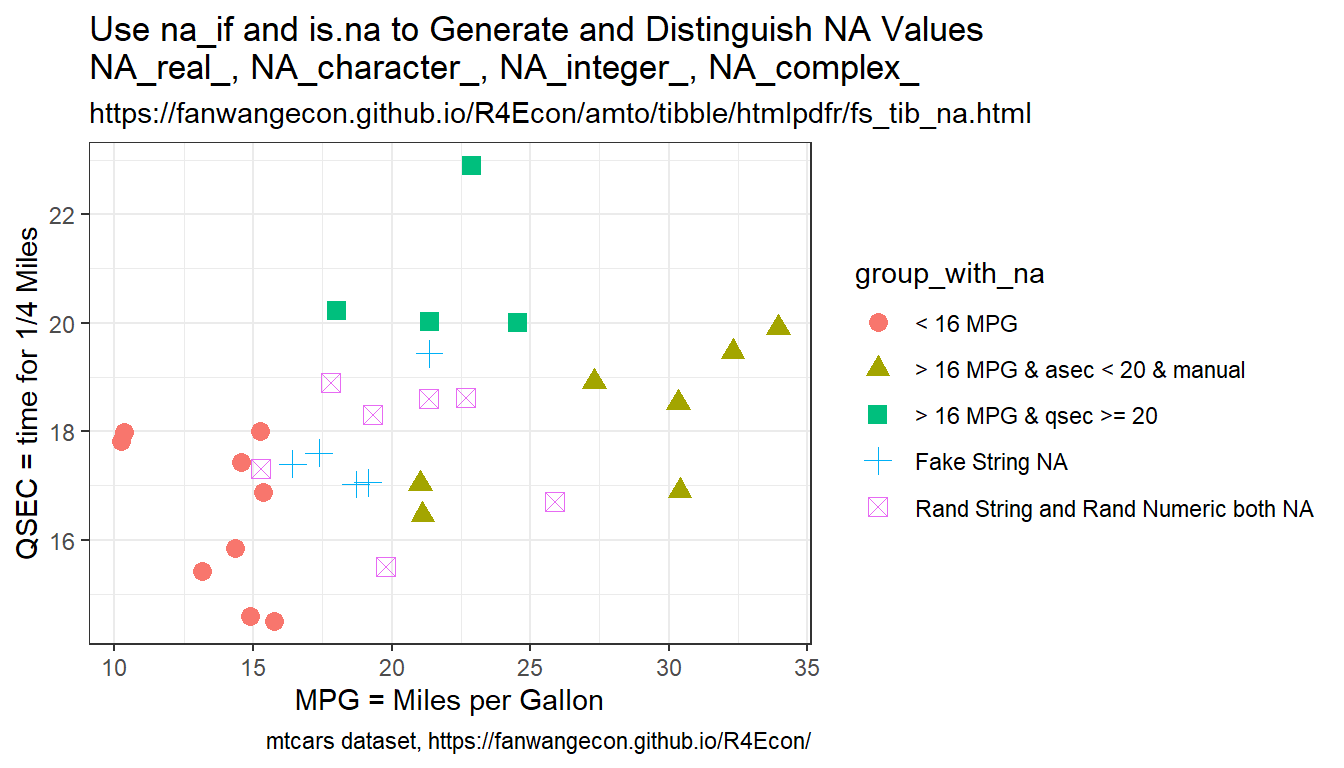

2.1.4.4 Approximate Values Comparison

r values almost the same
all.equal

From numeric approximation, often values are very close, and should be set to equal. Use isTRUE(all.equal). In the example below, we randomly generates four arrays. Two of the arrays have slightly higher variance, two arrays have slightly lower variance. They sd are to be 10 times below or 10 times above the tolerance comparison level. The values are not the same in any of the columns, but by allowing for almost true given some tolerance level, in the low standard deviation case, the values differences are within tolerance, so they are equal.

This is an essential issue when dealing with optimization results.

# Set tolerance
tol_lvl <- 1.5e-3
sd_lower_than_tol <- tol_lvl / 10
sd_higher_than_tol <- tol_lvl * 10

# larger SD
set.seed(123)
mt_runif_standard <- matrix(rnorm(10, mean = 0, sd = sd_higher_than_tol), nrow = 5, ncol = 2)

# small SD
set.seed(123)
mt_rnorm_small_sd <- matrix(rnorm(10, mean = 0, sd = sd_lower_than_tol), nrow = 5, ncol = 2)

# Generates Random Matirx
tb_rnorm_runif <- as_tibble(cbind(mt_rnorm_small_sd, mt_runif_standard))

# Are Variables the same, not for strict comparison
tb_rnorm_runif_approxi_same <- tb_rnorm_runif %>%
    mutate(
        V1_V2_ALMOST_SAME =
            case_when(
                isTRUE(all.equal(V1, V2, tolerance = tol_lvl)) ~
                    paste0("TOL=", sd_lower_than_tol, ", SAME ALMOST"),
                TRUE ~
                    paste0("TOL=", sd_lower_than_tol, ", NOT SAME ALMOST")
            )
    ) %>%
    mutate(
        V3_V4_ALMOST_SAME =
            case_when(
                isTRUE(all.equal(V3, V4, tolerance = tol_lvl)) ~
                    paste0("TOL=", sd_higher_than_tol, ", SAME ALMOST"),
                TRUE ~
                    paste0("TOL=", sd_higher_than_tol, ", NOT SAME ALMOST")
            )
    )

# Pring
kable(tb_rnorm_runif_approxi_same) %>% kable_styling_fc_wide()

V1	V2	V3	V4	V1_V2_ALMOST_SAME	V3_V4_ALMOST_SAME
-0.0000841	0.0002573	-0.0084071	0.0257260	TOL=0.00015, SAME ALMOST	TOL=0.015, NOT SAME ALMOST
-0.0000345	0.0000691	-0.0034527	0.0069137	TOL=0.00015, SAME ALMOST	TOL=0.015, NOT SAME ALMOST
0.0002338	-0.0001898	0.0233806	-0.0189759	TOL=0.00015, SAME ALMOST	TOL=0.015, NOT SAME ALMOST
0.0000106	-0.0001030	0.0010576	-0.0103028	TOL=0.00015, SAME ALMOST	TOL=0.015, NOT SAME ALMOST
0.0000194	-0.0000668	0.0019393	-0.0066849	TOL=0.00015, SAME ALMOST	TOL=0.015, NOT SAME ALMOST

2.1.5 String Dataframes

2.1.5.1 List of Strings to Tibble Datfare

There are several lists of strings, store them as variables in a dataframe.

# Sting data inputs
ls_st_abc <- c('a', 'b', 'c')
ls_st_efg <- c('e', 'f', 'g')
ls_st_opq <- c('o', 'p', 'q')
mt_str = cbind(ls_st_abc, ls_st_efg, ls_st_opq)

# Column Names
ar_st_varnames <- c('id','var1','var2','var3')

# Combine to tibble, add name col1, col2, etc.
tb_st_combine <- as_tibble(mt_str) %>%
  rowid_to_column(var = "id") %>%
  rename_all(~c(ar_st_varnames))

# Display
kable(tb_st_combine) %>% kable_styling_fc()

id	var1	var2	var3
1	a	e	o
2	b	f	p
3	c	g	q

2.1.5.2 Find and Replace

Find and Replace in Dataframe.

# if string value is contained in variable
("bridex.B" %in% (df.reg.out.all$vars_var.y))
# if string value is not contained in variable:
# 1. type is variable name
# 2. Toyota|Mazda are strings to be excluded
filter(mtcars, !grepl('Toyota|Mazda', type))

# filter does not contain string
rs_hgt_prot_log_tidy %>% filter(!str_detect(term, 'prot'))

2.2 Counting Observation

2.2.1 Counting and Tabulations

2.2.1.1 Tabulate Two Categorial Variables

First, we tabulate a dataset, and show categories as rows, and display frequencies.

# We use the mtcars dataset
tb_tab_joint <- mtcars %>%
    group_by(gear, am) %>%
    tally()
# Display
tb_tab_joint %>%
    kable(caption = "cross tabulation, stacked") %>%
    kable_styling_fc()

Table 2.4: cross tabulation, stacked
gear	am	n
3	0	15
4	0	4
4	1	8
5	1	5

We can present this as cross tabs.

# We use the mtcars dataset
tb_cross_tab <- mtcars %>%
    group_by(gear, am) %>%
    tally() %>%
    spread(am, n)
# Display
tb_cross_tab %>%
    kable(caption = "cross tabulation") %>%
    kable_styling_fc()

Table 2.5: cross tabulation
gear	0	1
3	15	NA
4	4	8
5	NA	5

2.2.1.2 Tabulate Once Each Distinct Subgroup

We have two variables variables, am and mpg, the mpg values are not unique. We want to know how many unique mpg levels are there for each am group. We use the dplyr::distinct function to achieve this.

tb_dist_tab <- mtcars %>%
    # .keep_all to keep all variables
    distinct(am, mpg, .keep_all = TRUE) %>%
    group_by(am) %>%
    tally()
# Display
tb_dist_tab %>%
    kable(caption = "Tabulate distinct groups") %>%
    kable_styling_fc()

Table 2.6: Tabulate distinct groups
am	n
0	16
1	11

2.2.1.3 Expanding to Panel

There are \(N\) individuals, each observed for \(Y_i\) years. We start with a dataframe where individuals are the unit of observation, we expand this to a panel with a row for each of the years that the individual is in the survey for.

Algorithm:

generate testing frame, the individual attribute dataset with invariant information over panel
uncount, duplicate rows by years in survey
group and generate sorted index
add indiviual specific stat year to index

First, we construct the dataframe where each row is an individual.

# 1. Array of Years in the Survey
ar_years_in_survey <- c(2, 3, 1, 10, 2, 5)
ar_start_yaer <- c(1, 2, 3, 1, 1, 1)
ar_end_year <- c(2, 4, 3, 10, 2, 5)
mt_combine <- cbind(ar_years_in_survey, ar_start_yaer, ar_end_year)

# This is the individual attribute dataset, attributes that are invariant acrosss years
tb_indi_attributes <- as_tibble(mt_combine) %>% rowid_to_column(var = "ID")

# Display
tb_indi_attributes %>%
    head(10) %>%
    kable() %>%
    kable_styling_fc()

ID	ar_years_in_survey	ar_start_yaer	ar_end_year
1	2	1	2
2	3	2	4
3	1	3	3
4	10	1	10
5	2	1	2
6	5	1	5

Second, we change the dataframe so that each unit of observation is an individual in an year. This means we will duplicate the information in the prior table, so if an individual appears for 4 years in the survey, we will now have four rows for this individual. We generate a new variable that is the calendar year. This is now a panel dataset.

# 2. Sort and generate variable equal to sorted index
tb_indi_panel <- tb_indi_attributes %>% uncount(ar_years_in_survey)

# 3. Panel now construct exactly which year in survey, note that all needed is sort index
# Note sorting not needed, all rows identical now
tb_indi_panel <- tb_indi_panel %>%
    group_by(ID) %>%
    mutate(yr_in_survey = row_number())

tb_indi_panel <- tb_indi_panel %>%
    mutate(calendar_year = yr_in_survey + ar_start_yaer - 1)

# Show results Head 10
tb_indi_panel %>%
    head(10) %>%
    kable() %>%
    kable_styling_fc()

ID	ar_start_yaer	ar_end_year	yr_in_survey	calendar_year
1	1	2	1	1
1	1	2	2	2
2	2	4	1	2
2	2	4	2	3
2	2	4	3	4
3	3	3	1	3
4	1	10	1	1
4	1	10	2	2
4	1	10	3	3
4	1	10	4	4

2.3 Sorting, Indexing, Slicing

2.3.1 Sorting

2.3.1.1 Generate Sorted Index within Group with Repeating Values

There is a variable, sort by this variable, then generate index from 1 to N representing sorted values of this index. If there are repeating values, still assign index, different index each value.

r generate index sort
dplyr mutate equals index

# Sort and generate variable equal to sorted index
df_iris <- iris %>% arrange(Sepal.Length) %>%
              mutate(Sepal.Len.Index = row_number()) %>%
              select(Sepal.Length, Sepal.Len.Index, everything())

# Show results Head 10
df_iris %>% head(10) %>%
  kable() %>%
  kable_styling_fc_wide()

Sepal.Length	Sepal.Len.Index	Sepal.Width	Petal.Length	Petal.Width	Species
4.3	1	3.0	1.1	0.1	setosa
4.4	2	2.9	1.4	0.2	setosa
4.4	3	3.0	1.3	0.2	setosa
4.4	4	3.2	1.3	0.2	setosa
4.5	5	2.3	1.3	0.3	setosa
4.6	6	3.1	1.5	0.2	setosa
4.6	7	3.4	1.4	0.3	setosa
4.6	8	3.6	1.0	0.2	setosa
4.6	9	3.2	1.4	0.2	setosa
4.7	10	3.2	1.3	0.2	setosa

2.3.1.2 Populate Value from Lowest Index to All other Rows

We would like to calculate for example the ratio of each individual’s highest to the the person with the lowest height in a dataset. We first need to generated sorted index from lowest to highest, and then populate the lowest height to all rows, and then divide.

Search Terms:

r spread value to all rows from one row
r other rows equal to the value of one row
Conditional assignment of one variable to the value of one of two other variables
dplyr mutate conditional
dplyr value from one row to all rows
dplyr mutate equal to value in another cell

Links:

see: dplyr rank
see: dplyr case_when

2.3.1.2.1 Short Method: mutate and min

We just want the lowest value to be in its own column, so that we can compute various statistics using the lowest value variable and the original variable.

# 1. Sort
df_iris_m1 <- iris %>% mutate(Sepal.Len.Lowest.all = min(Sepal.Length)) %>%
                select(Sepal.Length, Sepal.Len.Lowest.all, everything())


# Show results Head 10
df_iris_m1 %>% head(10) %>%
  kable() %>%
  kable_styling_fc_wide()

Sepal.Length	Sepal.Len.Lowest.all	Sepal.Width	Petal.Length	Petal.Width	Species
5.1	4.3	3.5	1.4	0.2	setosa
4.9	4.3	3.0	1.4	0.2	setosa
4.7	4.3	3.2	1.3	0.2	setosa
4.6	4.3	3.1	1.5	0.2	setosa
5.0	4.3	3.6	1.4	0.2	setosa
5.4	4.3	3.9	1.7	0.4	setosa
4.6	4.3	3.4	1.4	0.3	setosa
5.0	4.3	3.4	1.5	0.2	setosa
4.4	4.3	2.9	1.4	0.2	setosa
4.9	4.3	3.1	1.5	0.1	setosa

2.3.1.2.2 Long Method: row_number and case_when

This is the long method, using row_number, and case_when. The benefit of this method is that it generates several intermediate variables that might be useful. And the key final step is to set a new variable (A=Sepal.Len.Lowest.all) equal to another variable’s (B=Sepal.Length’s) value at the index that satisfies condition based a third variable (C=Sepal.Len.Index).

# 1. Sort
# 2. generate index
# 3. value at lowest index (case_when)
# 4. spread value from lowest index to other rows
# Note step 4 does not require step 3
df_iris_m2 <- iris %>% arrange(Sepal.Length) %>%
              mutate(Sepal.Len.Index = row_number()) %>%
              mutate(Sepal.Len.Lowest.one =
                       case_when(row_number()==1 ~ Sepal.Length)) %>%
              mutate(Sepal.Len.Lowest.all =
                       Sepal.Length[Sepal.Len.Index==1]) %>%
              select(Sepal.Length, Sepal.Len.Index,
                     Sepal.Len.Lowest.one, Sepal.Len.Lowest.all)


# Show results Head 10
df_iris_m2 %>% head(10) %>%
  kable() %>%
  kable_styling_fc_wide()

Sepal.Length	Sepal.Len.Index	Sepal.Len.Lowest.one	Sepal.Len.Lowest.all
4.3	1	4.3	4.3
4.4	2	NA	4.3
4.4	3	NA	4.3
4.4	4	NA	4.3
4.5	5	NA	4.3
4.6	6	NA	4.3
4.6	7	NA	4.3
4.6	8	NA	4.3
4.6	9	NA	4.3
4.7	10	NA	4.3

2.3.1.3 Generate Sorted Index based on Deviations

Generate Positive and Negative Index based on Ordered Deviation from some Number.

There is a variable that is continuous, substract a number from this variable, and generate index based on deviations. Think of the index as generating intervals indicating where the value lies. 0th index indicates the largest value in sequence that is smaller than or equal to number \(x\), 1st index indicates the smallest value in sequence that is larger than number \(x\).

The solution below is a little bit convoluated and long, there is likely a much quicker way. The process below shows various intermediary outputs that help arrive at deviation index Sepal.Len.Devi.Index from initial sorted index Sepal.Len.Index.

search:

dplyr arrange ignore na
dplyr index deviation from order number sequence
dplyr index below above
dplyr index order below above value

# 1. Sort and generate variable equal to sorted index
# 2. Plus or minus deviations from some value
# 3. Find the zero, which means, the number closests to zero including zero from the negative side
# 4. Find the index at the highest zero and below deviation point
# 5. Difference of zero index and original sorted index
sc_val_x <- 4.65
df_iris_deviate <- iris %>% arrange(Sepal.Length) %>%
              mutate(Sepal.Len.Index = row_number()) %>%
              mutate(Sepal.Len.Devi = (Sepal.Length - sc_val_x)) %>%
              mutate(Sepal.Len.Devi.Neg =
                       case_when(Sepal.Len.Devi <= 0 ~ (-1)*(Sepal.Len.Devi))) %>%
              arrange((Sepal.Len.Devi.Neg), desc(Sepal.Len.Index)) %>%
              mutate(Sepal.Len.Index.Zero =
                       case_when(row_number() == 1 ~ Sepal.Len.Index)) %>%
              mutate(Sepal.Len.Devi.Index =
                       Sepal.Len.Index - Sepal.Len.Index.Zero[row_number() == 1]) %>%
              arrange(Sepal.Len.Index) %>%
              select(Sepal.Length, Sepal.Len.Index, Sepal.Len.Devi,
                     Sepal.Len.Devi.Neg, Sepal.Len.Index.Zero, Sepal.Len.Devi.Index)


# Show results Head 10
df_iris_deviate %>% head(20) %>%
  kable() %>%
  kable_styling_fc_wide()

Sepal.Length	Sepal.Len.Index	Sepal.Len.Devi	Sepal.Len.Devi.Neg	Sepal.Len.Index.Zero	Sepal.Len.Devi.Index
4.3	1	-0.35	0.35	NA	-8
4.4	2	-0.25	0.25	NA	-7
4.4	3	-0.25	0.25	NA	-6
4.4	4	-0.25	0.25	NA	-5
4.5	5	-0.15	0.15	NA	-4
4.6	6	-0.05	0.05	NA	-3
4.6	7	-0.05	0.05	NA	-2
4.6	8	-0.05	0.05	NA	-1
4.6	9	-0.05	0.05	9	0
4.7	10	0.05	NA	NA	1
4.7	11	0.05	NA	NA	2
4.8	12	0.15	NA	NA	3
4.8	13	0.15	NA	NA	4
4.8	14	0.15	NA	NA	5
4.8	15	0.15	NA	NA	6
4.8	16	0.15	NA	NA	7
4.9	17	0.25	NA	NA	8
4.9	18	0.25	NA	NA	9
4.9	19	0.25	NA	NA	10
4.9	20	0.25	NA	NA	11

2.3.2 Group, Sort and Slice

2.3.2.1 Sort in Ascending and Descending Orders

We sort the mtcars dataset, sorting in ascending order by cyl, and in descending order by mpg. Using arrange, desc(disp) means sorting the disp variable in descending order. In the table shown below, cyc is increasing, and disp id decreasing within each cyc group.

kable(mtcars %>%
  arrange(cyl, desc(disp)) %>%
    # Select and filter to reduce display clutter
    select(cyl, disp, mpg)) %>%
  kable_styling_fc()

	cyl	disp	mpg
Merc 240D	4	146.7	24.4
Merc 230	4	140.8	22.8
Volvo 142E	4	121.0	21.4
Porsche 914-2	4	120.3	26.0
Toyota Corona	4	120.1	21.5
Datsun 710	4	108.0	22.8
Lotus Europa	4	95.1	30.4
Fiat X1-9	4	79.0	27.3
Fiat 128	4	78.7	32.4
Honda Civic	4	75.7	30.4
Toyota Corolla	4	71.1	33.9
Hornet 4 Drive	6	258.0	21.4
Valiant	6	225.0	18.1
Merc 280	6	167.6	19.2
Merc 280C	6	167.6	17.8
Mazda RX4	6	160.0	21.0
Mazda RX4 Wag	6	160.0	21.0
Ferrari Dino	6	145.0	19.7
Cadillac Fleetwood	8	472.0	10.4
Lincoln Continental	8	460.0	10.4
Chrysler Imperial	8	440.0	14.7
Pontiac Firebird	8	400.0	19.2
Hornet Sportabout	8	360.0	18.7
Duster 360	8	360.0	14.3
Ford Pantera L	8	351.0	15.8
Camaro Z28	8	350.0	13.3
Dodge Challenger	8	318.0	15.5
AMC Javelin	8	304.0	15.2
Maserati Bora	8	301.0	15.0
Merc 450SE	8	275.8	16.4
Merc 450SL	8	275.8	17.3
Merc 450SLC	8	275.8	15.2

2.3.2.2 Get Highest Values from Groups

There is a dataframe with a grouping variable with N unique values, for example N classes. Find the top three highest scoring students from each class. In the example below, group by cyl and get the cars with the highest and second highest mpg cars in each cyl group.

# use mtcars: slice_head gets the lowest sorted value
df_groupby_top_mpg <- mtcars %>%
  rownames_to_column(var = "car") %>%
  arrange(cyl, desc(mpg)) %>%
  group_by(cyl) %>%
  slice_head(n=3) %>%
  select(car, cyl, mpg, disp, hp)

# display
kable(df_groupby_top_mpg) %>% kable_styling_fc()

car	cyl	mpg	disp	hp
Toyota Corolla	4	33.9	71.1	65
Fiat 128	4	32.4	78.7	66
Honda Civic	4	30.4	75.7	52
Hornet 4 Drive	6	21.4	258.0	110
Mazda RX4	6	21.0	160.0	110
Mazda RX4 Wag	6	21.0	160.0	110
Pontiac Firebird	8	19.2	400.0	175
Hornet Sportabout	8	18.7	360.0	175
Merc 450SL	8	17.3	275.8	180

2.3.2.3 Differences in Within-group Sorted Value

We first take the largest N values in M groups, then we difference between the ranked top values in each group.

We have N classes, and M students in each class. We first select the 3 students with the highest scores from each class, then we take the difference between 1st and 2nd, and the difference between the 2nd and the 3rd students.

Note that when are using descending sort, so lead means the next value in descending sequencing, and lag means the last value which was higher in descending order.

# We use what we just created in the last block.
df_groupby_top_mpg_diff <- df_groupby_top_mpg %>%
  group_by(cyl) %>%
  mutate(mpg_diff_higher_minus_lower = mpg - lead(mpg)) %>%
  mutate(mpg_diff_lower_minus_higher = mpg - lag(mpg))

# display
kable(df_groupby_top_mpg_diff)  %>% kable_styling_fc()

car	cyl	mpg	disp	hp	mpg_diff_higher_minus_lower	mpg_diff_lower_minus_higher
Toyota Corolla	4	33.9	71.1	65	1.5	NA
Fiat 128	4	32.4	78.7	66	2.0	-1.5
Honda Civic	4	30.4	75.7	52	NA	-2.0
Hornet 4 Drive	6	21.4	258.0	110	0.4	NA
Mazda RX4	6	21.0	160.0	110	0.0	-0.4
Mazda RX4 Wag	6	21.0	160.0	110	NA	0.0
Pontiac Firebird	8	19.2	400.0	175	0.5	NA
Hornet Sportabout	8	18.7	360.0	175	1.4	-0.5
Merc 450SL	8	17.3	275.8	180	NA	-1.4

2.4 Advanced Group Aggregation

2.4.1 Cumulative Statistics within Group

2.4.1.1 Cumulative Mean

There is a dataset where there are different types of individuals, perhaps household size, that is the grouping variable. Within each group, we compute the incremental marginal propensity to consume for each additional check. We now also want to know the average propensity to consume up to each check considering all allocated checks. We needed to calculatet this for Nygaard, Sørensen and Wang (2021). This can be dealt with by using the cumall function.

Use the df_hgt_wgt as the testing dataset. In the example below, group by individual id, sort by survey month, and cumulative mean over the protein variable.

In the protein example

First select the testing dataset and variables.

# Load the REconTools Dataset df_hgt_wgt
data("df_hgt_wgt")
# str(df_hgt_wgt)

# Select several rows
df_hgt_wgt_sel <- df_hgt_wgt %>% 
  filter(S.country == "Cebu") %>%
  select(indi.id, svymthRound, prot)

Second, arrange, groupby, and cumulative mean. The protein variable is protein for each survey month, from month 2 to higher as babies grow. The protein intake observed is increasing quickly, hence, the cumulative mean is lower than the observed value for the survey month of the baby.

# Group by indi.id and sort by protein
df_hgt_wgt_sel_cummean <- df_hgt_wgt_sel %>%
  arrange(indi.id, svymthRound) %>%
  group_by(indi.id) %>%
  mutate(prot_cummean = cummean(prot))

# display results
REconTools::ff_summ_percentiles(df_hgt_wgt_sel_cummean)
# display results
df_hgt_wgt_sel_cummean %>% filter(indi.id %in% c(17, 18)) %>% 
  kable() %>% kable_styling_fc()

indi.id	svymthRound	prot	prot_cummean
17	0	0.5	0.5000000
17	2	0.7	0.6000000
17	4	0.5	0.5666667
17	6	0.5	0.5500000
17	8	6.1	1.6600000
17	10	5.0	2.2166667
17	12	6.4	2.8142857
17	14	20.1	4.9750000
17	16	20.1	6.6555556
17	18	23.0	8.2900000
17	20	24.9	9.8000000
17	22	20.1	10.6583333
17	24	10.1	10.6153846
17	102	NA	NA
17	138	NA	NA
17	187	NA	NA
17	224	NA	NA
17	258	NA	NA
18	0	1.2	1.2000000
18	2	4.7	2.9500000
18	4	17.2	7.7000000
18	6	18.6	10.4250000
18	8	NA	NA
18	10	16.8	NA
18	12	NA	NA
18	14	NA	NA
18	16	NA	NA
18	18	NA	NA
18	20	NA	NA
18	22	15.7	NA
18	24	22.5	NA
18	102	NA	NA
18	138	NA	NA
18	187	NA	NA
18	224	NA	NA
18	258	NA	NA

Third, in the basic implementation above, if an incremental month has NA, no values computed at that point or after. This is the case for individual 18 above. To ignore NA, we have, from this. Note how results for individual 18 changes.

# https://stackoverflow.com/a/49906718/8280804
# Group by indi.id and sort by protein
df_hgt_wgt_sel_cummean_noNA <- df_hgt_wgt_sel %>%
  arrange(indi.id, svymthRound) %>%
  group_by(indi.id, isna = is.na(prot)) %>%
  mutate(prot_cummean = ifelse(isna, NA, cummean(prot)))

# display results
df_hgt_wgt_sel_cummean_noNA %>% filter(indi.id %in% c(17, 18)) %>% 
  kable() %>% kable_styling_fc()

indi.id	svymthRound	prot	isna	prot_cummean
17	0	0.5	FALSE	0.5000000
17	2	0.7	FALSE	0.6000000
17	4	0.5	FALSE	0.5666667
17	6	0.5	FALSE	0.5500000
17	8	6.1	FALSE	1.6600000
17	10	5.0	FALSE	2.2166667
17	12	6.4	FALSE	2.8142857
17	14	20.1	FALSE	4.9750000
17	16	20.1	FALSE	6.6555556
17	18	23.0	FALSE	8.2900000
17	20	24.9	FALSE	9.8000000
17	22	20.1	FALSE	10.6583333
17	24	10.1	FALSE	10.6153846
17	102	NA	TRUE	NA
17	138	NA	TRUE	NA
17	187	NA	TRUE	NA
17	224	NA	TRUE	NA
17	258	NA	TRUE	NA
18	0	1.2	FALSE	1.2000000
18	2	4.7	FALSE	2.9500000
18	4	17.2	FALSE	7.7000000
18	6	18.6	FALSE	10.4250000
18	8	NA	TRUE	NA
18	10	16.8	FALSE	11.7000000
18	12	NA	TRUE	NA
18	14	NA	TRUE	NA
18	16	NA	TRUE	NA
18	18	NA	TRUE	NA
18	20	NA	TRUE	NA
18	22	15.7	FALSE	12.3666667
18	24	22.5	FALSE	13.8142857
18	102	NA	TRUE	NA
18	138	NA	TRUE	NA
18	187	NA	TRUE	NA
18	224	NA	TRUE	NA
18	258	NA	TRUE	NA

2.4.2 Groups Statistics

2.4.2.1 Aggrgate Groups only Unique Group and Count

There are two variables that are numeric, we want to find all the unique groups of these two variables in a dataset and count how many times each unique group occurs

r unique occurrence of numeric groups
How to add count of unique values by group to R data.frame

# Numeric value combinations unique Groups
vars.group <- c('hgt0', 'wgt0')

# dataset subsetting
df_use <- df_hgt_wgt %>% select(!!!syms(c(vars.group))) %>%
            mutate(hgt0 = round(hgt0/5)*5, wgt0 = round(wgt0/2000)*2000) %>%
            drop_na()

# Group, count and generate means for each numeric variables
# mutate_at(vars.group, funs(as.factor(.))) %>%
df.group.count <- df_use %>% group_by(!!!syms(vars.group)) %>%
                    arrange(!!!syms(vars.group)) %>%
                    summarise(n_obs_group=n())

# Show results Head 10
df.group.count %>% kable() %>% kable_styling_fc()

hgt0	wgt0	n_obs_group
40	2000	122
45	2000	4586
45	4000	470
50	2000	9691
50	4000	13106
55	2000	126
55	4000	1900
60	6000	18

2.4.2.2 Aggrgate Groups only Unique Group Show up With Means

Several variables that are grouping identifiers. Several variables that are values which mean be unique for each group members. For example, a Panel of income for N households over T years with also household education information that is invariant over time. Want to generate a dataset where the unit of observation are households, rather than household years. Take average of all numeric variables that are household and year specific.

A complicating factor potentially is that the number of observations differ within group, for example, income might be observed for all years for some households but not for other households.

r dplyr aggregate group average
Aggregating and analyzing data with dplyr
column can’t be modified because it is a grouping variable
see also: Aggregating and analyzing data with dplyr

# In the df_hgt_wgt from R4Econ, there is a country id, village id,
# and individual id, and various other statistics
vars.group <- c('S.country', 'vil.id', 'indi.id')
vars.values <- c('hgt', 'momEdu')

# dataset subsetting
df_use <- df_hgt_wgt %>% select(!!!syms(c(vars.group, vars.values)))

# Group, count and generate means for each numeric variables
df.group <- df_use %>% group_by(!!!syms(vars.group)) %>%
            arrange(!!!syms(vars.group)) %>%
            summarise_if(is.numeric,
                         funs(mean = mean(., na.rm = TRUE),
                              sd = sd(., na.rm = TRUE),
                              n = sum(is.na(.)==0)))

# Show results Head 10
df.group %>% head(10) %>%
  kable() %>%
  kable_styling_fc_wide()

S.country	vil.id	indi.id	hgt_mean	momEdu_mean	hgt_sd	hgt_n	momEdu_n
Cebu	1	1	61.80000	5.3	9.520504	7	18
Cebu	1	2	68.86154	7.1	9.058931	13	18
Cebu	1	3	80.45882	9.4	29.894231	17	18
Cebu	1	4	88.10000	13.9	35.533166	18	18
Cebu	1	5	97.70556	11.3	41.090366	18	18
Cebu	1	6	87.49444	7.3	35.586439	18	18
Cebu	1	7	90.79412	10.4	38.722385	17	18
Cebu	1	8	68.45385	13.5	10.011961	13	18
Cebu	1	9	86.21111	10.4	35.126057	18	18
Cebu	1	10	87.67222	10.5	36.508127	18	18

# Show results Head 10
df.group %>% tail(10) %>%
  kable() %>%
  kable_styling_fc_wide()

S.country	vil.id	indi.id	hgt_mean	momEdu_mean	hgt_sd	momEdu_sd	hgt_n
Guatemala	14	2014	66.97000	NaN	8.967974	NA	10
Guatemala	14	2015	71.71818	NaN	11.399984	NA	11
Guatemala	14	2016	66.33000	NaN	9.490352	NA	10
Guatemala	14	2017	76.40769	NaN	14.827871	NA	13
Guatemala	14	2018	74.55385	NaN	12.707846	NA	13
Guatemala	14	2019	70.47500	NaN	11.797390	NA	12
Guatemala	14	2020	60.28750	NaN	7.060036	NA	8
Guatemala	14	2021	84.96000	NaN	15.446193	NA	10
Guatemala	14	2022	79.38667	NaN	15.824749	NA	15
Guatemala	14	2023	66.50000	NaN	8.613113	NA	8

2.4.3 One Variable Group Summary

There is a categorical variable (based on one or the interaction of multiple variables), there is a continuous variable, obtain statistics for the continuous variable conditional on the categorical variable, but also unconditionally.

Store results in a matrix, but also flatten results wide to row with appropriate keys/variable-names for all group statistics.

Pick which statistics to be included in final wide row

2.4.3.1 Build Program

# Single Variable Group Statistics (also generate overall statistics)
ff_summ_by_group_summ_one <- function(
  df, vars.group, var.numeric, str.stats.group = 'main',
  str.stats.specify = NULL, boo.overall.stats = TRUE){
  
  # List of statistics
  # https://rdrr.io/cran/dplyr/man/summarise.html
  strs.center <- c('mean', 'median')
  strs.spread <- c('sd', 'IQR', 'mad')
  strs.range <- c('min', 'max')
  strs.pos <- c('first', 'last')
  strs.count <- c('n_distinct')
  
  # Grouping of Statistics
  if (missing(str.stats.specify)) {
    if (str.stats.group == 'main') {
      strs.all <- c('mean', 'min', 'max', 'sd')
    }
    if (str.stats.group == 'all') {
      strs.all <- c(strs.center, strs.spread, strs.range, strs.pos, strs.count)
    }
  } else {
    strs.all <- str.stats.specify
  }
  
  # Start Transform
  df <- df %>% drop_na() %>% 
    mutate(!!(var.numeric) := as.numeric(!!sym(var.numeric)))
  
  # Overall Statistics
  if (boo.overall.stats) {
    df.overall.stats <- df %>% 
      summarize_at(vars(var.numeric), funs(!!!strs.all))
    if (length(strs.all) == 1) {
      # give it a name, otherwise if only one stat, name of stat not saved
      df.overall.stats <- df.overall.stats %>% 
        rename(!!strs.all := !!sym(var.numeric))
    }
    names(df.overall.stats) <- 
      paste0(var.numeric, '.', names(df.overall.stats))
  }
  
  # Group Sort
  df.select <- df %>%
    group_by(!!!syms(vars.group)) %>%
    arrange(!!!syms(c(vars.group, var.numeric)))
  
  # Table of Statistics
  df.table.grp.stats <- df.select %>% 
    summarize_at(vars(var.numeric), funs(!!!strs.all))
  
  # Add Stat Name
  if (length(strs.all) == 1) {
    # give it a name, otherwise if only one stat, name of stat not saved
    df.table.grp.stats <- df.table.grp.stats %>% 
      rename(!!strs.all := !!sym(var.numeric))
  }
  
  
  # Row of Statistics
  str.vars.group.combine <- paste0(vars.group, collapse='_')
  if (length(vars.group) == 1) {
    df.row.grp.stats <- df.table.grp.stats %>%
      mutate(!!(str.vars.group.combine) := 
               paste0(var.numeric, '.',
                      vars.group, '.g',
                      (!!!syms(vars.group)))) %>%
      gather(variable, value, -one_of(vars.group)) %>%
      unite(str.vars.group.combine, c(str.vars.group.combine, 'variable')) %>%
      spread(str.vars.group.combine, value)
  } else {
    df.row.grp.stats <- df.table.grp.stats %>% 
      mutate(vars.groups.combine := 
               paste0(paste0(vars.group, collapse='.')),
             !!(str.vars.group.combine) := 
               paste0(interaction(!!!(syms(vars.group))))) %>%
      mutate(!!(str.vars.group.combine) := 
               paste0(var.numeric, '.', vars.groups.combine, '.',
                      (!!sym(str.vars.group.combine)))) %>%
      ungroup() %>%
      select(-vars.groups.combine, -one_of(vars.group)) %>%
      gather(variable, value, -one_of(str.vars.group.combine)) %>%
      unite(str.vars.group.combine, c(str.vars.group.combine, 'variable')) %>%
      spread(str.vars.group.combine, value)
  }
  
  # Clean up name strings
  names(df.table.grp.stats) <- 
    gsub(x = names(df.table.grp.stats),pattern = "_", replacement = "\\.")
  names(df.row.grp.stats) <- 
    gsub(x = names(df.row.grp.stats),pattern = "_", replacement = "\\.")
  
  # Return
  list.return <- 
    list(df_table_grp_stats = df.table.grp.stats, 
         df_row_grp_stats = df.row.grp.stats)
  
  # Overall Statistics, without grouping
  if (boo.overall.stats) {
    df.row.stats.all <- c(df.row.grp.stats, df.overall.stats)
    list.return <- append(list.return, 
                          list(df_overall_stats = df.overall.stats,
                               df_row_stats_all = df.row.stats.all))
  }
  
  # Return
  return(list.return)
  
}

2.4.3.2 Test

Load data and test

# Library
library(tidyverse)

# Load Sample Data
setwd('C:/Users/fan/R4Econ/_data/')
df <- read_csv('height_weight.csv')

2.4.3.2.1 Function Testing By Gender Groups

Need two variables, a group variable that is a factor, and a numeric

vars.group <- 'sex'
var.numeric <- 'hgt'

df.select <- df %>% select(one_of(vars.group, var.numeric)) %>% drop_na()

Main Statistics:

# Single Variable Group Statistics
ff_summ_by_group_summ_one(
  df.select, vars.group = vars.group, var.numeric = var.numeric, 
  str.stats.group = 'main')$df_table_grp_stats

Specify Two Specific Statistics:

ff_summ_by_group_summ_one(
  df.select, vars.group = vars.group, var.numeric = var.numeric, 
  str.stats.specify = c('mean', 'sd'))$df_table_grp_stats

Specify One Specific Statistics:

ff_summ_by_group_summ_one(
  df.select, vars.group = vars.group, var.numeric = var.numeric, 
  str.stats.specify = c('mean'))$df_table_grp_stats

2.4.3.2.2 Function Testing By Country and Gender Groups

Need two variables, a group variable that is a factor, and a numeric. Now joint grouping variables.

vars.group <- c('S.country', 'sex')
var.numeric <- 'hgt'

df.select <- df %>% select(one_of(vars.group, var.numeric)) %>% drop_na()

Main Statistics:

ff_summ_by_group_summ_one(
  df.select, vars.group = vars.group, var.numeric = var.numeric, 
  str.stats.group = 'main')$df_table_grp_stats

Specify Two Specific Statistics:

ff_summ_by_group_summ_one(
  df.select, vars.group = vars.group, var.numeric = var.numeric, 
  str.stats.specify = c('mean', 'sd'))$df_table_grp_stats

Specify One Specific Statistics:

ff_summ_by_group_summ_one(
  df.select, vars.group = vars.group, var.numeric = var.numeric, 
  str.stats.specify = c('mean'))$df_table_grp_stats

2.4.4 Nested within Group Stats

By Multiple within Individual Groups Variables, Averages for All Numeric Variables within All Groups of All Group Variables (Long to very Wide). Suppose you have an individual level final outcome. The individual is observed for N periods, where each period the inputs differ. What inputs impacted the final outcome?

Suppose we can divide N periods in which the individual is in the data into a number of years, a number of semi-years, a number of quarters, or uneven-staggered lengths. We might want to generate averages across individuals and within each of these different possible groups averages of inputs.

Then we want to version of the data where each row is an individual, one of the variables is the final outcome, and the other variables are these different averages: averages for the 1st, 2nd, 3rd year in which indivdiual is in data, averages for 1st, …, final quarter in which indivdiual is in data.

2.4.4.1 Build Function

This function takes as inputs:

vars.not.groups2avg: a list of variables that are not the within-indivdiual or across-individual grouping variables, but the variables we want to average over. Withnin indivdiual grouping averages will be calculated for these variables using the not-listed variables as within indivdiual groups (excluding vars.indi.grp groups).
vars.indi.grp: a list or individual variables, and also perhaps villages, province, etc id variables that are higher than individual ID. Note the groups are are ACROSS individual higher level group variables.
the remaining variables are all within individual grouping variables.

the function output is a dataframe:

each row is an individual
initial variables individual ID and across individual groups from vars.indi.grp.
other variables are all averages for the variables in vars.not.groups2avg
- if there are 2 within individual group variables, and the first has 3 groups (years), the second has 6 groups (semi-years), then there would be 9 average variables.
- each average variables has the original variable name from vars.not.groups2avg plus the name of the within individual grouping variable, and at the end ‘c_x’, where x is a integer representing the category within the group (if 3 years, x=1, 2, 3)

# Data Function
# https://fanwangecon.github.io/R4Econ/summarize/summ/ByGroupsSummWide.html
f.by.groups.summ.wide <- function(df.groups.to.average,
                                  vars.not.groups2avg,
                                  vars.indi.grp = c('S.country','ID'),
                                  display=TRUE) {

# 1. generate categoricals for full year (m.12), half year (m.6), quarter year (m.4)
# 2. generate categoricals also for uneven years (m12t14) using 
#  stagger (+2 rather than -1)
# 3. reshape wide to long, so that all categorical date groups appear in var=value,
    # and categories in var=variable
# 4. calculate mean for all numeric variables for all date groups
# 5. combine date categorical variable and value, single var:
    # m.12.c1= first year average from m.12 averaging

######## ######## ######## ######## #######
# Step 1
######## ######## ######## ######## #######
# 1. generate categoricals for full year (m.12), half year (m.6), quarter year (m.4)
# 2. generate categoricals also for uneven years (m12t14) using stagger 
#  (+2 rather than -1)

######## ######## ######## ######## #######
# S2: reshape wide to long, so that all categorical date groups appear in var=value,
# and categories in var=variable; calculate mean for all 
# numeric variables for all date groups
######## ######## ######## ######## #######
df.avg.long <- df.groups.to.average %>%
       gather(variable, value, -one_of(c(vars.indi.grp,
                                         vars.not.groups2avg))) %>%
       group_by(!!!syms(vars.indi.grp), variable, value) %>%
       summarise_if(is.numeric, funs(mean(., na.rm = TRUE)))

if (display){
  dim(df.avg.long)
  options(repr.matrix.max.rows=10, repr.matrix.max.cols=20)
  print(df.avg.long)
}

######## ######## ######## ######## #######
# S3 combine date categorical variable and value, single var:
# m.12.c1= first year average from m.12 averaging; to do this make 
# data even longer first
######## ######## ######## ######## #######

# We already have the averages, but we want them to show up as variables,
    # mean for each group of each variable.
df.avg.allvars.wide <- df.avg.long %>%
   ungroup() %>%
   mutate(all_m_cate = paste0(variable, '_c', value)) %>%
   select(all_m_cate, everything(), -variable, -value) %>%
   gather(variable, value, -one_of(vars.indi.grp), -all_m_cate) %>%
   unite('var_mcate', variable, all_m_cate) %>%
   spread(var_mcate, value)

if (display){
  dim(df.avg.allvars.wide)
  options(repr.matrix.max.rows=10, repr.matrix.max.cols=10)
  print(df.avg.allvars.wide)
}

return(df.avg.allvars.wide)
}

2.4.4.2 Test Program

In our sample dataset, the number of nutrition/height/income etc information observed within each country and month of age group are different. We have a panel dataset for children observed over different months of age.

We have two key grouping variables: 1. country: data are observed for guatemala and cebu 2. month-age (survey month round=svymthRound): different months of age at which each individual child is observed

A child could be observed for many months, or just a few months. A child’s height information could be observed for more months-of-age than nutritional intake information. We eventually want to run regressions where the outcome is height/weight and the input is nutrition. The regressions will be at the month-of-age level. We need to know how many times different variables are observed at the month-of-age level.

# Library
library(tidyverse)

# Load Sample Data
setwd('C:/Users/fan/R4Econ/_data/')
df <- read_csv('height_weight.csv')

2.4.4.2.1 Generate Within Individual Groups

In the data, children are observed for different number of months since birth. We want to calculate quarterly, semi-year, annual, etc average nutritional intakes. First generate these within-individual grouping variables. We can also generate uneven-staggered calendar groups as shown below.

mth.var <- 'svymthRound'
df.groups.to.average<- df %>%
        filter(!!sym(mth.var) >= 0 & !!sym(mth.var) <= 24)  %>%
        mutate(m12t24=(floor((!!sym(mth.var) - 12) %/% 14) + 1),
               m8t24=(floor((!!sym(mth.var) - 8) %/% 18) + 1),
               m12 = pmax((floor((!!sym(mth.var)-1) %/% 12) + 1), 1),
               m6 = pmax((floor((!!sym(mth.var)-1) %/% 6) + 1), 1),
               m3 = pmax((floor((!!sym(mth.var)-1) %/% 3) + 1), 1))

# Show Results
options(repr.matrix.max.rows=30, repr.matrix.max.cols=20)
vars.arrange <- c('S.country','indi.id','svymthRound')
vars.groups.within.indi <- c('m12t24', 'm8t24', 'm12', 'm6', 'm3')
as.tibble(df.groups.to.average %>%
          group_by(!!!syms(vars.arrange)) %>%
          arrange(!!!syms(vars.arrange)) %>%
          select(!!!syms(vars.arrange), !!!syms(vars.groups.within.indi)))

2.4.4.2.2 Within Group Averages

With the within-group averages created, we can generate averages for all variables within these groups.

vars.not.groups2avg <- c('prot', 'cal')
vars.indi.grp <- c('S.country', 'indi.id')
vars.groups.within.indi <- c('m12t24', 'm8t24', 'm12', 'm6', 'm3')

df.groups.to.average.select <- df.groups.to.average %>%
                        select(one_of(c(vars.indi.grp,
                                        vars.not.groups2avg,
                                        vars.groups.within.indi)))
df.avg.allvars.wide <- f.by.groups.summ.wide(df.groups.to.average.select,
                                             vars.not.groups2avg,
                                             vars.indi.grp, display=FALSE)

This is the tabular version of results

dim(df.avg.allvars.wide)

## [1] 2023   38

names(df.avg.allvars.wide)

##  [1] "S.country"      "indi.id"        "cal_m12_c1"     "cal_m12_c2"    
##  [5] "cal_m12t24_c0"  "cal_m12t24_c1"  "cal_m3_c1"      "cal_m3_c2"     
##  [9] "cal_m3_c3"      "cal_m3_c4"      "cal_m3_c5"      "cal_m3_c6"     
## [13] "cal_m3_c7"      "cal_m3_c8"      "cal_m6_c1"      "cal_m6_c2"     
## [17] "cal_m6_c3"      "cal_m6_c4"      "cal_m8t24_c0"   "cal_m8t24_c1"  
## [21] "prot_m12_c1"    "prot_m12_c2"    "prot_m12t24_c0" "prot_m12t24_c1"
## [25] "prot_m3_c1"     "prot_m3_c2"     "prot_m3_c3"     "prot_m3_c4"    
## [29] "prot_m3_c5"     "prot_m3_c6"     "prot_m3_c7"     "prot_m3_c8"    
## [33] "prot_m6_c1"     "prot_m6_c2"     "prot_m6_c3"     "prot_m6_c4"    
## [37] "prot_m8t24_c0"  "prot_m8t24_c1"

df.avg.allvars.wide[1:20,] %>% kable() %>% kable_styling_fc_wide()

S.country	indi.id	cal_m12_c1	cal_m12_c2	cal_m12t24_c0	cal_m12t24_c1	cal_m3_c1	cal_m3_c2	cal_m3_c3	cal_m3_c4	cal_m3_c5	cal_m3_c6	cal_m3_c7	cal_m3_c8	cal_m6_c1	cal_m6_c2	cal_m6_c3	cal_m6_c4	cal_m8t24_c0	cal_m8t24_c1	prot_m12_c1	prot_m12_c2	prot_m12t24_c0	prot_m12t24_c1	prot_m3_c1	prot_m3_c2	prot_m3_c3	prot_m3_c4	prot_m3_c5	prot_m3_c6	prot_m3_c7	prot_m3_c8	prot_m6_c1	prot_m6_c2	prot_m6_c3	prot_m6_c4	prot_m8t24_c0	prot_m8t24_c1
Cebu	1	132.15714	NaN	97.08333	342.6000	9.10	95.50	85.3	315.30	NaN	NaN	NaN	NaN	52.300	238.63333	NaN	NaN	52.300	238.6333	5.3571429	NaN	4.3666667	11.300000	0.65	3.65	2.6	13.15	NaN	NaN	NaN	NaN	2.150	9.6333333	NaN	NaN	2.150	9.633333
Cebu	2	90.72857	255.6500	81.46667	240.0286	83.35	12.30	155.1	144.35	228.0	152.85	305.0	347.60	47.825	147.93333	177.9000	333.4000	47.825	219.7444	3.1857143	8.550000	2.7333333	8.171429	3.20	1.25	5.2	4.10	5.4	5.15	7.7	13.95	2.225	4.4666667	5.233333	11.866667	2.225	7.188889
Cebu	3	96.80000	658.8167	31.56667	634.4429	0.50	28.85	57.0	280.95	459.3	549.95	612.0	890.85	14.675	206.30000	519.7333	797.9000	14.675	507.9778	4.5000000	21.116667	1.6833333	21.157143	1.05	2.15	2.3	11.40	18.5	18.05	18.0	27.05	1.600	8.3666667	18.200000	24.033333	1.600	16.866667
Cebu	4	27.45714	371.7000	24.55000	325.0143	4.50	25.95	39.4	45.95	221.2	271.00	581.3	442.85	15.225	43.76667	254.4000	489.0000	15.225	262.3889	0.8714286	6.850000	0.9000000	5.971429	0.75	1.10	1.2	0.60	1.8	4.85	10.1	9.75	0.925	0.8000000	3.833333	9.866667	0.925	4.833333
Cebu	5	101.34286	1080.8500	79.15000	959.9429	14.10	143.80	71.3	161.15	452.6	1345.20	1178.1	1082.00	78.950	131.20000	1047.6667	1114.0333	78.950	764.3000	2.4000000	19.483333	2.3166667	17.114286	1.35	3.00	3.4	2.35	7.1	23.15	24.5	19.50	2.175	2.7000000	17.800000	21.166667	2.175	13.888889
Cebu	6	185.35714	521.5333	162.23333	493.3286	23.85	184.70	169.1	355.65	653.4	506.50	416.8	523.00	104.275	293.46667	555.4667	487.6000	104.275	445.5111	8.4000000	15.116667	7.3833333	15.028571	0.85	7.40	9.8	16.25	26.8	14.10	11.4	12.15	4.125	14.1000000	18.333333	11.900000	4.125	14.777778
Cebu	7	157.25714	570.9800	145.50000	513.7833	8.30	137.80	407.8	200.40	390.6	637.10	688.1	569.55	73.050	269.53333	513.8500	609.0667	73.050	457.9375	3.3000000	20.440000	2.7833333	18.100000	0.95	1.70	8.6	4.60	16.4	23.00	21.5	20.65	1.325	5.9333333	19.700000	20.933333	1.325	15.000000
Cebu	8	471.92857	844.8333	379.20000	871.0429	158.95	423.00	417.5	861.05	691.3	897.95	637.1	972.35	290.975	713.20000	829.0667	860.6000	290.975	800.9556	13.6857143	32.716667	11.0166667	32.285714	3.90	11.35	10.8	27.25	42.7	26.45	25.8	37.45	7.625	21.7666667	31.866667	33.566667	7.625	29.066667
Cebu	9	32.27143	415.2167	16.58333	373.9571	5.05	10.40	15.1	89.95	142.4	203.60	753.2	594.25	7.725	65.00000	183.2000	647.2333	7.725	298.4778	0.9571429	18.283333	0.9166667	15.842857	0.50	0.50	0.5	2.10	4.2	10.85	39.5	22.15	0.500	1.5666667	8.633333	27.933333	0.500	12.711111
Cebu	10	67.18571	395.2500	68.58333	347.1857	9.55	26.40	164.6	116.90	296.6	303.00	385.1	541.90	17.975	132.80000	300.8667	489.6333	17.975	307.7667	2.0428571	8.466667	1.9333333	7.642857	0.85	0.50	4.9	3.35	7.5	6.05	9.2	11.00	0.675	3.8666667	6.533333	10.400000	0.675	6.933333
Cebu	11	14.90000	245.3833	11.80000	215.1143	0.50	5.20	30.0	31.45	126.2	223.05	239.6	330.20	2.850	30.96667	190.7667	300.0000	2.850	173.9111	1.0285714	6.833333	1.1166667	5.928571	0.80	1.70	1.2	0.50	3.6	6.35	7.3	8.70	1.250	0.7333333	5.433333	8.233333	1.250	4.800000
Cebu	12	453.61429	745.6833	419.51667	733.1857	325.60	483.65	463.0	546.90	766.8	676.85	998.5	677.55	404.625	518.93333	706.8333	784.5333	404.625	670.1000	14.7714286	22.133333	14.1666667	21.600000	7.40	13.60	26.6	17.40	18.6	20.35	25.6	23.95	10.500	20.4666667	19.766667	24.500000	10.500	21.577778
Cebu	13	47.51429	210.2500	36.81667	196.1714	17.45	40.00	28.5	94.60	216.9	195.15	281.3	186.50	28.725	72.56667	202.4000	218.1000	28.725	164.3556	1.9571429	6.800000	1.6666667	6.357143	0.70	1.50	2.1	3.60	8.3	4.75	6.2	8.40	1.100	3.1000000	5.933333	7.666667	1.100	5.566667
Cebu	14	608.85714	924.5833	527.30000	949.3857	259.05	554.30	688.1	973.60	525.5	1039.60	800.0	1071.40	406.675	878.43333	868.2333	980.9333	406.675	909.2000	24.6714286	28.050000	23.0833333	28.928571	15.05	28.85	32.6	26.15	12.7	29.75	29.5	33.30	21.950	28.3000000	24.066667	32.033333	21.950	28.133333
Cebu	15	74.67143	440.0833	64.21667	396.8429	62.40	39.60	80.1	119.30	292.5	237.45	607.8	632.65	51.000	106.23333	255.8000	624.3667	51.000	328.8000	2.2571429	10.633333	1.6333333	9.971429	1.65	0.90	1.5	4.60	9.4	5.80	13.6	14.60	1.275	3.5666667	7.000000	14.266667	1.275	8.277778
Cebu	16	128.45714	519.9333	90.50000	496.5429	4.80	11.00	205.3	331.15	290.8	354.50	563.3	778.25	7.900	289.20000	333.2667	706.6000	7.900	443.0222	4.6857143	18.083333	4.1000000	16.671429	0.65	2.70	8.7	8.70	7.8	12.95	25.9	24.45	1.675	8.7000000	11.233333	24.933333	1.675	14.955556
Cebu	17	130.78571	718.8667	97.48333	663.4000	5.50	7.80	249.9	319.50	774.6	892.90	551.9	600.45	6.650	296.30000	853.4667	584.2667	6.650	578.0111	2.8142857	19.716667	2.2166667	17.814286	0.60	0.50	6.1	5.70	20.1	21.55	24.9	15.10	0.550	5.8333333	21.066667	18.366667	0.550	15.088889
Cebu	18	172.64000	497.9500	172.64000	497.9500	29.60	234.40	NaN	335.20	NaN	NaN	NaN	497.95	132.000	335.20000	NaN	497.9500	132.000	443.7000	11.7000000	19.100000	11.7000000	19.100000	2.95	17.90	NaN	16.80	NaN	NaN	NaN	19.10	10.425	16.8000000	NaN	19.100000	10.425	18.333333
Cebu	19	74.45714	314.7333	80.10000	275.5714	3.65	95.70	171.3	75.60	131.3	350.50	304.6	375.75	49.675	107.50000	277.4333	352.0333	49.675	245.6556	2.5428571	10.466667	2.8833333	9.042857	0.50	2.95	6.7	2.10	3.4	11.40	12.3	12.15	1.725	3.6333333	8.733333	12.200000	1.725	8.188889
Cebu	20	110.90000	583.2000	80.51667	541.7714	7.30	120.65	77.8	221.30	391.2	582.10	466.1	738.85	63.975	173.46667	518.4667	647.9333	63.975	446.6222	3.2000000	16.966667	2.1833333	15.871429	0.50	3.85	2.7	5.50	7.9	20.15	11.8	20.90	2.175	4.5666667	16.066667	17.866667	2.175	12.833333

2.5 Distributional Statistics

2.5.1 Histogram

2.5.1.1 Generate Test Score Dataset

r generate text string as csv
r tibble matrix hand input

First, we will generate a test score dataset, directly from string. Below we type line by line a dataset with four variables in comma separated (csv) format, where the first row includes the variables names. These texts could be stored in a separate file, or they could be directly included in code and read in as csv

2.5.1.1.1 A Dataset with only Two Continuous Variable

ar_test_scores_ec3 <- c(107.72,101.28,105.92,109.31,104.27,110.27,91.92846154,81.8,109.0071429,103.07,98.97923077,101.91,96.49,97.79923077,99.07846154,99.17,103.51,112.2225,101.2964286,94.5,98.92,97.09,93.83989011,97.36304945,80.34,65.74,85.275,82.19708791,86.53758242,86.2025,86.63,82.57392857,83.66,79.76,75.55642857,86.32571429,66.41,76.06,44.225,82.28,47.77392857,70.005,69.13769231,73.52571429,60.51,56.04)
ar_test_scores_ec1 <- c(101.72,101.28,99.92,103.31,100.27,104.27,90.23615385,77.8,103.4357143,97.07,93.13307692,95.91,92.49,93.95307692,95.38615385,97.17,99.51,100.3475,95.83214286,92.5,94.92,91.09,90.4332967,93.52101648,80.34,59.74,79.525,77.67236264,81.59252747,82.3275,80.63,76.98464286,81.66,79.76,70.59214286,82.46857143,66.41,74.06,40.475,76.28,44.18464286,66.255,65.59923077,69.66857143,60.51,56.04)
mt_test_scores <- cbind(ar_test_scores_ec1, ar_test_scores_ec3)
ar_st_varnames <- c('course_total_ec1p','course_total_ec3p')
tb_final_twovar <- as_tibble(mt_test_scores) %>% rename_all(~c(ar_st_varnames))
summary(tb_final_twovar)

##  course_total_ec1p course_total_ec3p
##  Min.   : 40.48    Min.   : 44.23   
##  1st Qu.: 76.46    1st Qu.: 79.91   
##  Median : 86.35    Median : 89.28   
##  Mean   : 83.88    Mean   : 87.90   
##  3rd Qu.: 95.89    3rd Qu.:100.75   
##  Max.   :104.27    Max.   :112.22

ff_summ_percentiles(df = tb_final_twovar, bl_statsasrows = TRUE, col2varname = FALSE)

2.5.1.1.2 A Dataset with one Continuous Variable and Histogram

ar_final_scores <- c(94.28442509,95.68817475,97.25219512,77.89268293,95.08795497,93.27380863,92.3,84.25317073,86.08642991,84.69219512,71.43634146,76.21365854,71.68878049,77.46142589,79.29579268,43.7285453,63.80634146,67.92994774,100.8980488,100.0857143,99.93073171,98.4102439,97.93,97.10359756,96.97121951,96.60292683,96.23317073,93.92243902,93.82243902,92.75390244,92.65775261,92.20444653,91.73463415,90.38321161,89.37414634,86.95932458,79.58686411,78.70878049,77.2497561,76.88195122,76.52987805,74.72114313,74.27488676,71.30268293,63.70256098,37.90426829,2.292682927)
mt_test_scores <- cbind(seq(1,length(ar_final_scores)), ar_final_scores)
ar_st_varnames <- c('index', 'course_final')
tb_onevar <- as_tibble(mt_test_scores) %>% rename_all(~c(ar_st_varnames))
summary(tb_onevar)

##      index       course_final    
##  Min.   : 1.0   Min.   :  2.293  
##  1st Qu.:12.5   1st Qu.: 76.372  
##  Median :24.0   Median : 86.959  
##  Mean   :24.0   Mean   : 82.415  
##  3rd Qu.:35.5   3rd Qu.: 94.686  
##  Max.   :47.0   Max.   :100.898

ff_summ_percentiles(df = tb_onevar, bl_statsasrows = TRUE, col2varname = FALSE)

2.5.1.1.3 A Dataset with Multiple Variables

#load in data empirically by hand
txt_test_data <- "init_prof, later_prof, class_id, exam_score
 'SW', 'SW', 1, 102
 'SW', 'SW', 1, 102
 'SW', 'SW', 1, 101
 'SW', 'SW', 1, 100
 'SW', 'SW', 1, 100
 'SW', 'SW', 1, 99
 'SW', 'SW', 1, 98.5
 'SW', 'SW', 1, 98.5
 'SW', 'SW', 1, 97
 'SW', 'SW', 1, 95
 'SW', 'SW', 1, 94
 'SW', 'SW', 1, 91
 'SW', 'SW', 1, 91
 'SW', 'SW', 1, 90
 'SW', 'SW', 1, 89
 'SW', 'SW', 1, 88.5
 'SW', 'SW', 1, 88
 'SW', 'SW', 1, 87
 'SW', 'SW', 1, 87
 'SW', 'SW', 1, 87
 'SW', 'SW', 1, 86
 'SW', 'SW', 1, 86
 'SW', 'SW', 1, 84
 'SW', 'SW', 1, 82
 'SW', 'SW', 1, 78.5
 'SW', 'SW', 1, 76
 'SW', 'SW', 1, 72
 'SW', 'SW', 1, 70.5
 'SW', 'SW', 1, 67.5
 'SW', 'SW', 1, 67.5
 'SW', 'SW', 1, 67
 'SW', 'SW', 1, 63.5
 'SW', 'SW', 1, 60
 'SW', 'SW', 1, 59
 'SW', 'SW', 1, 44.5
 'SW', 'SW', 1, 44
 'SW', 'SW', 1, 42.5
 'SW', 'SW', 1, 40.5
 'SW', 'SW', 1, 40.5
 'SW', 'SW', 1, 36.5
 'SW', 'SW', 1, 35.5
 'SW', 'SW', 1, 21.5
 'SW', 'SW', 1, 4
 'MP', 'MP', 2, 105
 'MP', 'MP', 2, 103
 'MP', 'MP', 2, 102
 'MP', 'MP', 2, 101
 'MP', 'MP', 2, 101
 'MP', 'MP', 2, 100.5
 'MP', 'MP', 2, 100
 'MP', 'MP', 2, 99
 'MP', 'MP', 2, 97
 'MP', 'MP', 2, 97
 'MP', 'MP', 2, 97
 'MP', 'MP', 2, 97
 'MP', 'MP', 2, 96
 'MP', 'MP', 2, 95
 'MP', 'MP', 2, 91
 'MP', 'MP', 2, 89
 'MP', 'MP', 2, 85
 'MP', 'MP', 2, 84
 'MP', 'MP', 2, 84
 'MP', 'MP', 2, 84
 'MP', 'MP', 2, 83.5
 'MP', 'MP', 2, 82.5
 'MP', 'MP', 2, 81.5
 'MP', 'MP', 2, 80.5
 'MP', 'MP', 2, 80
 'MP', 'MP', 2, 77
 'MP', 'MP', 2, 77
 'MP', 'MP', 2, 75
 'MP', 'MP', 2, 75
 'MP', 'MP', 2, 71
 'MP', 'MP', 2, 70
 'MP', 'MP', 2, 68
 'MP', 'MP', 2, 63
 'MP', 'MP', 2, 56
 'MP', 'MP', 2, 56
 'MP', 'MP', 2, 55.5
 'MP', 'MP', 2, 49.5
 'MP', 'MP', 2, 48.5
 'MP', 'MP', 2, 47.5
 'MP', 'MP', 2, 44.5
 'MP', 'MP', 2, 34.5
 'MP', 'MP', 2, 29.5
 'CA', 'MP', 3, 103
 'CA', 'MP', 3, 103
 'CA', 'MP', 3, 101
 'CA', 'MP', 3, 96.5
 'CA', 'MP', 3, 93.5
 'CA', 'MP', 3, 93
 'CA', 'MP', 3, 93
 'CA', 'MP', 3, 92
 'CA', 'MP', 3, 90
 'CA', 'MP', 3, 90
 'CA', 'MP', 3, 89
 'CA', 'MP', 3, 86.5
 'CA', 'MP', 3, 84.5
 'CA', 'MP', 3, 83
 'CA', 'MP', 3, 83
 'CA', 'MP', 3, 82
 'CA', 'MP', 3, 78
 'CA', 'MP', 3, 75
 'CA', 'MP', 3, 74.5
 'CA', 'MP', 3, 70
 'CA', 'MP', 3, 54.5
 'CA', 'MP', 3, 52
 'CA', 'MP', 3, 50
 'CA', 'MP', 3, 42
 'CA', 'MP', 3, 36.5
 'CA', 'MP', 3, 28
 'CA', 'MP', 3, 26
 'CA', 'MP', 3, 11
 'CA', 'SN', 4, 103
 'CA', 'SN', 4, 103
 'CA', 'SN', 4, 102
 'CA', 'SN', 4, 102
 'CA', 'SN', 4, 101
 'CA', 'SN', 4, 100
 'CA', 'SN', 4, 98
 'CA', 'SN', 4, 98
 'CA', 'SN', 4, 98
 'CA', 'SN', 4, 95
 'CA', 'SN', 4, 95
 'CA', 'SN', 4, 92.5
 'CA', 'SN', 4, 92
 'CA', 'SN', 4, 91
 'CA', 'SN', 4, 90
 'CA', 'SN', 4, 85.5
 'CA', 'SN', 4, 84
 'CA', 'SN', 4, 82.5
 'CA', 'SN', 4, 81
 'CA', 'SN', 4, 77.5
 'CA', 'SN', 4, 77
 'CA', 'SN', 4, 72
 'CA', 'SN', 4, 71.5
 'CA', 'SN', 4, 69
 'CA', 'SN', 4, 68.5
 'CA', 'SN', 4, 68
 'CA', 'SN', 4, 67
 'CA', 'SN', 4, 65.5
 'CA', 'SN', 4, 62.5
 'CA', 'SN', 4, 62
 'CA', 'SN', 4, 61.5
 'CA', 'SN', 4, 61
 'CA', 'SN', 4, 57.5
 'CA', 'SN', 4, 54
 'CA', 'SN', 4, 52.5
 'CA', 'SN', 4, 51
 'CA', 'SN', 4, 50.5
 'CA', 'SN', 4, 50
 'CA', 'SN', 4, 49
 'CA', 'SN', 4, 43
 'CA', 'SN', 4, 39.5
 'CA', 'SN', 4, 32.5
 'CA', 'SN', 4, 25.5
 'CA', 'SN', 4, 18"

csv_test_data = read.csv(text=txt_test_data, header=TRUE)
ar_st_varnames <- c('first_half_professor',
                    'second_half_professor',
                    'course_id', 'exam_score')
tb_test_data <- as_tibble(csv_test_data) %>% 
  rename_all(~c(ar_st_varnames))
summary(tb_test_data)

##  first_half_professor second_half_professor   course_id       exam_score    
##  Length:157           Length:157            Min.   :1.000   Min.   :  4.00  
##  Class :character     Class :character      1st Qu.:1.000   1st Qu.: 60.00  
##  Mode  :character     Mode  :character      Median :2.000   Median : 82.00  
##                                             Mean   :2.465   Mean   : 75.08  
##                                             3rd Qu.:4.000   3rd Qu.: 94.00  
##                                             Max.   :4.000   Max.   :105.00

2.5.1.2 Test Score Distributions

2.5.1.2.1 Histogram

ggplot(tb_final_twovar, aes(x=ar_test_scores_ec3)) +
  geom_histogram(bins=25) +
  labs(title = paste0('Sandbox: Final Distribution (Econ 2370, FW)'),
       caption = paste0('FW Section, formula:',
                        '0.3*exam1Perc + 0.3*exam2Perc + ',
                        '0.42*HWtotalPerc + 0.03*AttendancePerc \n',
                        '+ perfect attendance + 0.03 per Extra Credit')) +
  theme_bw()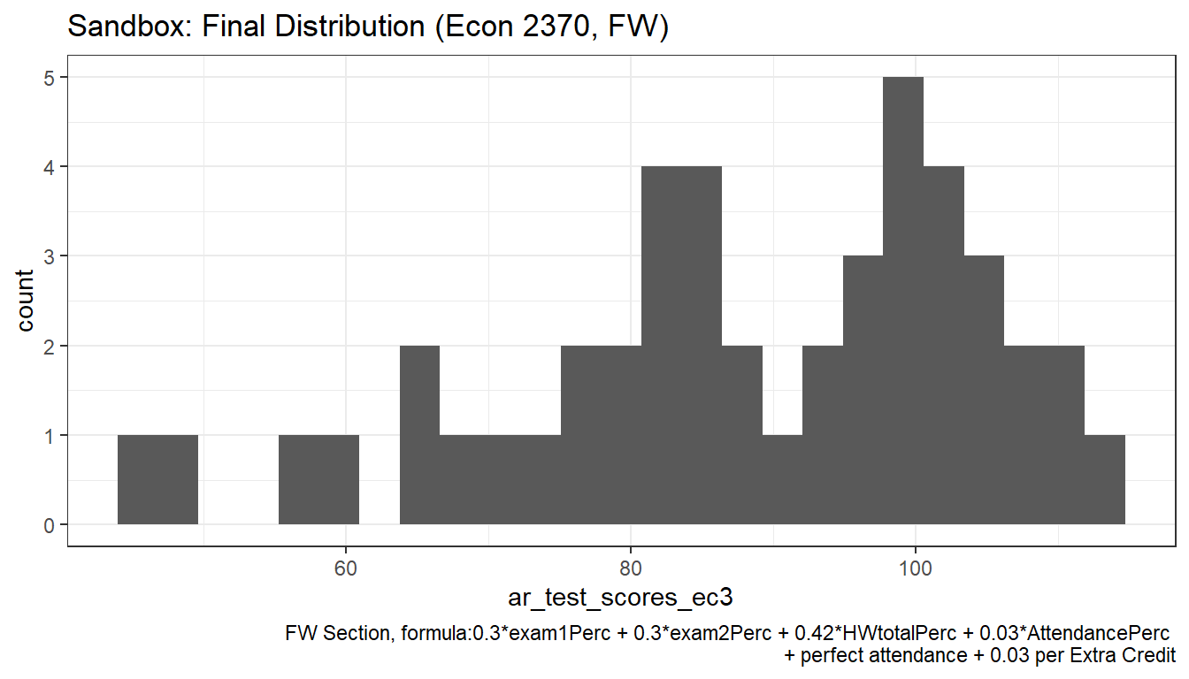

ggplot(tb_test_data, aes(x=exam_score)) +
  geom_histogram(bins=16) +
  labs(title = paste0('Exam Distribution'),
       caption = 'All Sections') +
  theme_bw()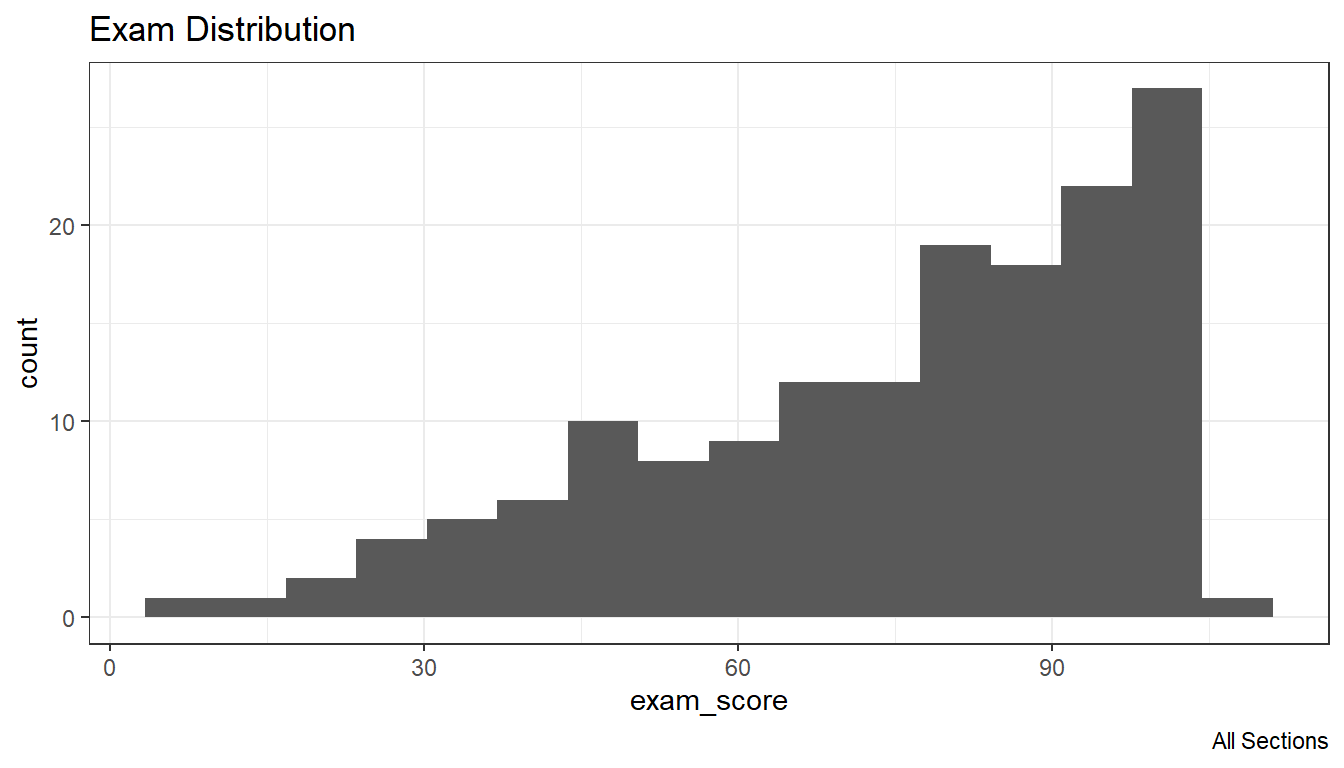

2.6 Summarize Multiple Variables

2.6.1 Apply Function Over Multiple Columns and Rows

2.6.1.1 Convert Subset of Variables to Numeric

Multiply a subset of variables all by 10. We use dplyr’s across function to achieve this.

Note that in the example below, we also use across with group by to include a string array of grouping by variables.

Note: “across() makes it easy to apply the same transformation to multiple columns, allowing you to use select() semantics inside in”data-masking” functions like summarise() and mutate().”

# grouping by variables
ar_st_groups <- c("gear", "carb")
# use across to conduct operation over multiple variables
mtcars_3var_times10 <- mtcars %>% 
  group_by(across(one_of(ar_st_groups))) %>%
  mutate(across(matches("mpg|cyl|disp"), ~ .x * 10)) %>%
  select(gear, carb, mpg, cyl, disp) %>% head(n=5)
# pring
# Multiply several variables by 10
kable(mtcars_3var_times10 %>% slice_head(n = 5)) %>% 
    kable_styling_fc()

gear	carb	mpg	cyl	disp
3	1	214	60	2580
3	2	187	80	3600
4	1	228	40	1080
4	4	210	60	1600
4	4	210	60	1600

2.6.1.2 Compute Row-specific Quantiles using Data Across Columns

We want to compute quantiles for each location, based on monthly variations in columns.

First, we generate a table with 12 columns (for months) and 3 rows (for locations).

# Generate data, 12 months as columns, and 
mt_data_rand <- matrix(rnorm(36, mean=0, sd=1), nrow=3, ncol=12)
it_rows <- seq(1, dim(mt_data_rand)[1])
it_cols <- seq(1, dim(mt_data_rand)[2])
# convert to table, column as month with leading 0
colnames(mt_data_rand) <- paste0('m', sprintf("%02d", it_cols))
tb_data_full <- as_tibble(mt_data_rand, rownames = NA) %>% 
    mutate(loc = paste0("loc", sprintf("%02d", row_number()))) %>%
    select(loc, everything())
# Display
kable(tb_data_full) %>% kable_styling_fc_wide()

loc	m01	m02	m03	m04	m05	m06	m07	m08	m09	m10	m11	m12
loc01	1.2240818	0.1106827	0.4978505	-0.4727914	-1.0260044	-1.6866933	-1.1381369	-0.2950715	0.8215811	-0.0619117	-0.6947070	2.168956
loc02	0.3598138	-0.5558411	-1.9666172	-1.0678237	-0.7288912	0.8377870	1.2538149	0.8951257	0.6886403	-0.3059627	-0.2079173	1.207962
loc03	0.4007715	1.7869131	0.7013559	-0.2179749	-0.6250393	0.1533731	0.4264642	0.8781335	0.5539177	-0.3804710	-1.2653964	-1.123109

Second, using apply to compute quantiles, row by row

# Extract the data components from the tibble, tibble has row and column names
tb_data_only <- tb_data_full %>% 
    column_to_rownames(var = "loc") %>% 
    select(contains("m"))
# Compute row specific quantiles
ar_quantiles_by_row <- apply(tb_data_only, 1, quantile, probs=0.75)
# Display
print(ar_quantiles_by_row)

##     loc01     loc02     loc03 
## 0.5787831 0.8521217 0.5907772

Third, generate matrix of two columns, ID and quantile.

# One particular quantil from location
tb_loc_quantile <- as_tibble(ar_quantiles_by_row) %>% 
    mutate(loc = names(ar_quantiles_by_row)) %>%
    rename(quantile = value) %>%
    select(loc, everything())
# Display
kable(tb_loc_quantile) %>% kable_styling_fc()

loc	quantile
loc01	0.5787831
loc02	0.8521217
loc03	0.5907772

2.6.1.3 Compute Row-specific Sums using Data Across Columns

We compute sum over several variables in the mtcars dataset. We will sum over several variables with shared prefix, after adding these prefix first. We introduce an NA value to make sure that we can sum ignoring NA

We sum using three different methods below: (1) purrr:reduce(), (2) base::rowSums(), (3) Manual sum. Note that the rowSums option is able to sum ignoring NA.

# we introduce NA value to first row
mtcars[1,1] <- NA
# Rename variables, and sum across
mtcars_rowsum <- mtcars %>%
    rename(stats_mpg = mpg, stats_cyl = cyl, stats_hp = hp) %>%
    mutate(
        cs_reduce = purrr::reduce(
            dplyr::pick(contains("stats")),
            `+`
        ),
        cs_rowsum = base::rowSums(
            dplyr::pick(contains("stats")),
            na.rm = TRUE
        ),
        cs_manual = stats_mpg + stats_cyl + stats_hp
    ) %>%
    select(matches("stats|cs"), gear)
# Display
# caption: "sum across columns"
kable(mtcars_rowsum %>% slice_head(n = 5)) %>% kable_styling_fc_wide()

	stats_mpg	stats_cyl	stats_hp	cs_reduce	cs_rowsum	cs_manual	gear
Mazda RX4	NA	6	110	NA	116.0	NA	4
Mazda RX4 Wag	21.0	6	110	137.0	137.0	137.0	4
Datsun 710	22.8	4	93	119.8	119.8	119.8	4
Hornet 4 Drive	21.4	6	110	137.4	137.4	137.4	3
Hornet Sportabout	18.7	8	175	201.7	201.7	201.7	3

See this discussion for column sum peed comparisons.

2.6.1.4 Sum Across Rows within Group

Following from the prior section, we now sum across rows within group.

# we introduce NA value to first row
# mtcars[1,1] <- NA
# Rename variables, and sum across
mtcars_grpsum <- mtcars_rowsum %>%  
    arrange(gear) %>% group_by(gear) %>%
    # srs = sum row sum
    mutate_at(vars(matches("stats|cs")), 
        .funs = list(gs = ~sum(., na.rm=TRUE))
    ) %>% 
    select(gear, matches("gs")) %>% 
    slice_head(n=1)
# Display
# caption: "gs = group sum, cs = col sum over the columns 
# with stats as prefix, sum across rows after col sum; gear = 4 
# difference for cs-rowsum-gs because it allowed for summing 
# ignoring NA for values across columns"
kable(mtcars_grpsum) %>% kable_styling_fc_wide()

gear	stats_mpg_gs	stats_cyl_gs	stats_hp_gs	cs_reduce_gs	cs_rowsum_gs	cs_manual_gs
3	241.6	112	2642	2995.6	2995.6	2995.6
4	273.4	56	1074	1287.4	1403.4	1287.4
5	106.9	30	978	1114.9	1114.9	1114.9

2.6.1.5 Replace NA for Multiple Variables

Replace some variables NA by some values, and other variables’ NAs by other values.

# Define
it_N <- 3
it_M <- 5
svr_id <- "date"

# NA dataframe, note need to define as NA_real_
# if define as NA, will not be able to replace with 99 column
# would be logical rather than double.
df_NA <- as_tibble(matrix(NA_real_, nrow = it_N, ncol = it_M)) %>%
    rowid_to_column(var = svr_id) %>%
    rename_at(
        vars(starts_with("V")),
        funs(str_replace(., "V", "var"))
    )
kable(df_NA) %>%
    kable_styling_fc()

date	var1	var2	var3	var4	var5
1	NA	NA	NA	NA	NA
2	NA	NA	NA	NA	NA
3	NA	NA	NA	NA	NA

# Replace NA
df_NA_replace <- df_NA %>%
    mutate_at(vars(one_of(c("var1", "var2"))), list(~ replace_na(., 0))) %>%
    mutate_at(vars(one_of(c("var3", "var5"))), list(~ replace_na(., 99)))

kable(df_NA_replace) %>%
    kable_styling_fc()

date	var3	var4	var5
1	99	NA	99
2	99	NA	99
3	99	NA	99

2.6.1.6 Cumulative Sum Multiple Variables

Each row is a different date, each column is the profit a firms earns on a date, we want to compute cumulatively how much a person is earning. Also renames variable names below jointly.

# Define
it_N <- 3
it_M <- 5
svr_id <- "date"

# random dataframe, daily profit of firms
# dp_fx: daily profit firm ID something
set.seed(123)
df_daily_profit <- as_tibble(matrix(rnorm(it_N * it_M), nrow = it_N, ncol = it_M)) %>%
    rowid_to_column(var = svr_id) %>%
    rename_at(
        vars(starts_with("V")),
        funs(str_replace(., "V", "dp_f"))
    )
kable(df_daily_profit) %>%
    kable_styling_fc()

date	dp_f1	dp_f2	dp_f3	dp_f4	dp_f5
1	-0.5604756	0.0705084	0.4609162	-0.4456620	0.4007715
2	-0.2301775	0.1292877	-1.2650612	1.2240818	0.1106827
3	1.5587083	1.7150650	-0.6868529	0.3598138	-0.5558411

# cumulative sum with suffix
df_cumu_profit_suffix <- df_daily_profit %>%
    mutate_at(vars(contains("dp_f")), .funs = list(cumu = ~ cumsum(.)))
kable(df_cumu_profit_suffix) %>%
    kable_styling_fc_wide()

date	dp_f1	dp_f2	dp_f3	dp_f4	dp_f5	dp_f1_cumu	dp_f2_cumu	dp_f3_cumu	dp_f4_cumu	dp_f5_cumu
1	-0.5604756	0.0705084	0.4609162	-0.4456620	0.4007715	-0.5604756	0.0705084	0.4609162	-0.4456620	0.4007715
2	-0.2301775	0.1292877	-1.2650612	1.2240818	0.1106827	-0.7906531	0.1997961	-0.8041450	0.7784198	0.5114542
3	1.5587083	1.7150650	-0.6868529	0.3598138	-0.5558411	0.7680552	1.9148611	-1.4909979	1.1382337	-0.0443870

# cumulative sum variables naming to prefix
df_cumu_profit <- df_cumu_profit_suffix %>%
    rename_at(vars(contains("_cumu")), list(~ paste("cp_f", gsub("_cumu", "", .), sep = ""))) %>%
    rename_at(vars(contains("cp_f")), list(~ gsub("dp_f", "", .)))
kable(df_cumu_profit) %>%
    kable_styling_fc_wide()

date	dp_f1	dp_f2	dp_f3	dp_f4	dp_f5	cp_f1	cp_f2	cp_f3	cp_f4	cp_f5
1	-0.5604756	0.0705084	0.4609162	-0.4456620	0.4007715	-0.5604756	0.0705084	0.4609162	-0.4456620	0.4007715
2	-0.2301775	0.1292877	-1.2650612	1.2240818	0.1106827	-0.7906531	0.1997961	-0.8041450	0.7784198	0.5114542
3	1.5587083	1.7150650	-0.6868529	0.3598138	-0.5558411	0.7680552	1.9148611	-1.4909979	1.1382337	-0.0443870

Sepal.Length	Sepal.Len.Index	Sepal.Len.Lowest.one	Sepal.Len.Lowest.all
4.3	1	4.3	4.3
4.4	2	NA	4.3
4.4	3	NA	4.3
4.4	4	NA	4.3
4.5	5	NA	4.3
4.6	6	NA	4.3
4.6	7	NA	4.3
4.6	8	NA	4.3
4.6	9	NA	4.3
4.7	10	NA	4.3

Sepal.Length	Sepal.Len.Index	Sepal.Len.Lowest.one	Sepal.Len.Lowest.all
4.3	1	4.3	4.3
4.4	2	NA	4.3
4.4	3	NA	4.3
4.4	4	NA	4.3
4.5	5	NA	4.3
4.6	6	NA	4.3
4.6	7	NA	4.3
4.6	8	NA	4.3
4.6	9	NA	4.3
4.7	10	NA	4.3

Sepal.Length	Sepal.Len.Index	Sepal.Len.Lowest.one	Sepal.Len.Lowest.all
4.3	1	4.3	4.3
4.4	2	NA	4.3
4.4	3	NA	4.3
4.4	4	NA	4.3
4.5	5	NA	4.3
4.6	6	NA	4.3
4.6	7	NA	4.3
4.6	8	NA	4.3
4.6	9	NA	4.3
4.7	10	NA	4.3