Chapter 4 Multi-dimensional Data Structures

4.1 Generate, Gather, Bind and Join

4.1.1 Generate Panel Structure

Go back to fan’s REconTools research support package, R4Econ examples page, PkgTestR packaging guide, or Stat4Econ course page.

4.1.1.1 Balanced Panel Skeleton

There are \(N\) individuals, each could be observed \(M\) times. In the example below, there are 3 students, each observed over 4 dates. This just uses the uncount function from tidyr.

# Define
it_N <- 3
it_M <- 5
svr_id <- 'student_id'
svr_date <- 'class_day'

# dataframe
df_panel_skeleton <- as_tibble(matrix(it_M, nrow=it_N, ncol=1)) %>%
  rowid_to_column(var = svr_id) %>%
  uncount(V1) %>%
  group_by(!!sym(svr_id)) %>% mutate(!!sym(svr_date) := row_number()) %>%
  ungroup()

# Print
kable(df_panel_skeleton) %>%
  kable_styling_fc()

student_id	class_day
1	1
1	2
1	3
1	4
1	5
2	1
2	2
2	3
2	4
2	5
3	1
3	2
3	3
3	4
3	5

4.1.1.2 Panel of Children with Height Growth

Given \(N\) individuals, each with \(G\) observations. There is an initial height variable and height grows every year. There are growth variables, variables for cumulative growth and variables for height at each age for each child.

Individuals are defined by gender (1 = female), race (1=asian), and birth height. Within individual yearly information includes height at each year of age.

# Define
it_N <- 5
it_M <- 3
svr_id <- 'indi_id'
svr_gender <- 'female'
svr_asian <- 'asian'
svr_age <- 'year_of_age'
# Define Height Related Variables
svr_brthgt <- 'birth_height'
svr_hgtgrow <- 'hgt_growth'
svr_hgtgrow_cumu <- 'hgt_growcumu'
svr_height <- 'height'

# panel dataframe following
set.seed(123)
df_panel_indiage <- as_tibble(matrix(it_M, nrow=it_N, ncol=1)) %>%
  mutate(!!sym(svr_gender) := rbinom(n(), 1, 0.5),
         !!sym(svr_asian) := rbinom(n(), 1, 0.5),
         !!sym(svr_brthgt) := rnorm(n(), mean=60,sd=3)) %>%
  uncount(V1) %>%
  group_by(!!sym(svr_gender), !!sym(svr_asian), !!sym(svr_brthgt)) %>%
  mutate(!!sym(svr_age) := row_number(),
         !!sym(svr_hgtgrow) := runif(n(), min=5, max=15),
         !!sym(svr_hgtgrow_cumu) := cumsum(!!sym(svr_hgtgrow)),
         !!sym(svr_height) := !!sym(svr_brthgt) + !!sym(svr_hgtgrow_cumu))  %>%
  ungroup()

# Add Height Index
kable(df_panel_indiage) %>% kable_styling_fc()

female	asian	birth_height	year_of_age	hgt_growth	hgt_growcumu	height
0	0	65.14520	1	13.895393	13.895393	79.04059
0	0	65.14520	2	11.928034	25.823427	90.96862
0	0	65.14520	3	11.405068	37.228495	102.37369
1	1	61.38275	1	11.907053	11.907053	73.28980
1	1	61.38275	2	12.954674	24.861727	86.24448
1	1	61.38275	3	5.246137	30.107864	91.49061
0	1	56.20482	1	14.942698	14.942698	71.14751
0	1	56.20482	2	11.557058	26.499756	82.70457
0	1	56.20482	3	12.085305	38.585060	94.78988
1	1	57.93944	1	6.471137	6.471137	64.41058
1	1	57.93944	2	14.630242	21.101379	79.04082
1	1	57.93944	3	14.022991	35.124369	93.06381
1	0	58.66301	1	10.440660	10.440660	69.10367
1	0	58.66301	2	10.941420	21.382081	80.04509
1	0	58.66301	3	7.891597	29.273678	87.93669

4.1.1.3 Create Group IDs

Given the dataframe just created, generate group IDs for each Gender and Race Groups. Given that both are binary, there can only be 4 unique groups.

# group id
svr_group_id <- 'female_asian_id'
# Define
ls_svr_group_vars <- c('female', 'asian')

# panel dataframe following
df_panel_indiage_id <- df_panel_indiage %>%
  arrange(!!!syms(ls_svr_group_vars)) %>%
  group_by(!!!syms(ls_svr_group_vars)) %>%
  mutate(!!sym(svr_group_id) := (row_number()==1)*1) %>%
  ungroup() %>%
  mutate(!!sym(svr_group_id) := cumsum(!!sym(svr_group_id))) %>%
  select(one_of(svr_group_id, ls_svr_group_vars), everything())

# Add Height Index
kable(df_panel_indiage_id) %>%
  kable_styling_fc_wide()

female_asian_id	female	asian	birth_height	year_of_age	hgt_growth	hgt_growcumu	height
1	0	0	65.14520	1	13.895393	13.895393	79.04059
1	0	0	65.14520	2	11.928034	25.823427	90.96862
1	0	0	65.14520	3	11.405068	37.228495	102.37369
2	0	1	56.20482	1	14.942698	14.942698	71.14751
2	0	1	56.20482	2	11.557058	26.499756	82.70457
2	0	1	56.20482	3	12.085305	38.585060	94.78988
3	1	0	58.66301	1	10.440660	10.440660	69.10367
3	1	0	58.66301	2	10.941420	21.382081	80.04509
3	1	0	58.66301	3	7.891597	29.273678	87.93669
4	1	1	61.38275	1	11.907053	11.907053	73.28980
4	1	1	61.38275	2	12.954674	24.861727	86.24448
4	1	1	61.38275	3	5.246137	30.107864	91.49061
4	1	1	57.93944	1	6.471137	6.471137	64.41058
4	1	1	57.93944	2	14.630242	21.101379	79.04082
4	1	1	57.93944	3	14.022991	35.124369	93.06381

4.1.2 Join Datasets

Go back to fan’s REconTools research support package, R4Econ examples page, PkgTestR packaging guide, or Stat4Econ course page.

4.1.2.1 Join Panel with Multiple Keys

We have two datasets, one for student enrollment, panel over time, but some students do not show up on some dates. The other is a skeleton panel with all student ID and all dates. Often we need to join dataframes together, and we need to join by the student ID and the panel time Key at the same time. When students show up, there is a quiz score for that day, so the joined panel should have as data column quiz score

Student count is \(N\), total dates are \(M\). First we generate two panels below, then we join by both keys using left_join. First, define dataframes:

# Define
it_N <- 4
it_M <- 3
svr_id <- 'sid'
svr_date <- 'classday'
svr_attend <- 'date_in_class'

# Panel Skeleton
df_panel_balanced_skeleton <- as_tibble(matrix(it_M, nrow=it_N, ncol=1)) %>%
  rowid_to_column(var = svr_id) %>%
  uncount(V1) %>%
  group_by(!!sym(svr_id)) %>% mutate(!!sym(svr_date) := row_number()) %>%
  ungroup()
# Print
kable(df_panel_balanced_skeleton) %>%
  kable_styling_fc()

sid	classday
1	1
1	2
1	3
2	1
2	2
2	3
3	1
3	2
3	3
4	1
4	2
4	3

# Smaller Panel of Random Days in School
set.seed(456)
df_panel_attend <- as_tibble(matrix(it_M, nrow=it_N, ncol=1)) %>%
  rowid_to_column(var = svr_id) %>%
  uncount(V1) %>%
  group_by(!!sym(svr_id)) %>% mutate(!!sym(svr_date) := row_number()) %>%
  ungroup() %>% mutate(in_class = case_when(rnorm(n(),mean=0,sd=1) < 0 ~ 1, TRUE ~ 0)) %>%
  filter(in_class == 1) %>% select(!!sym(svr_id), !!sym(svr_date)) %>%
  rename(!!sym(svr_attend) := !!sym(svr_date)) %>%
  mutate(dayquizscore = rnorm(n(),mean=80,sd=10))
# Print
kable(df_panel_attend) %>%
  kable_styling_fc()

sid	date_in_class	dayquizscore
1	1	89.88726
2	1	96.53929
2	2	65.59195
2	3	99.47356
4	2	97.36936

Second, now join dataframes:

# Join with explicit names
df_quiz_joined_multikey <- df_panel_balanced_skeleton %>%
  left_join(df_panel_attend,
            by=(c('sid'='sid', 'classday'='date_in_class')))

# Join with setname strings
df_quiz_joined_multikey_setnames <- df_panel_balanced_skeleton %>%
  left_join(df_panel_attend, by=setNames(c('sid', 'date_in_class'), c('sid', 'classday')))

# Print
kable(df_quiz_joined_multikey) %>%
  kable_styling_fc()

sid	classday	dayquizscore
1	1	89.88726
1	2	NA
1	3	NA
2	1	96.53929
2	2	65.59195
2	3	99.47356
3	1	NA
3	2	NA
3	3	NA
4	1	NA
4	2	97.36936
4	3	NA

kable(df_quiz_joined_multikey_setnames) %>%
  kable_styling_fc()

sid	classday	dayquizscore
1	1	89.88726
1	2	NA
1	3	NA
2	1	96.53929
2	2	65.59195
2	3	99.47356
3	1	NA
3	2	NA
3	3	NA
4	1	NA
4	2	97.36936
4	3	NA

4.1.2.2 Stack Panel Frames Together

There are multiple panel dataframe, each for different subsets of dates. All variable names and units of observations are identical. Use DPLYR bind_rows.

# Define
it_N <- 2 # Number of individuals
it_M <- 3 # Number of Months
svr_id <- 'sid'
svr_date <- 'date'

# Panel First Half of Year
df_panel_m1tom3 <- as_tibble(matrix(it_M, nrow=it_N, ncol=1)) %>%
  rowid_to_column(var = svr_id) %>%
  uncount(V1) %>%
  group_by(!!sym(svr_id)) %>% mutate(!!sym(svr_date) := row_number()) %>%
  ungroup()

# Panel Second Half of Year
df_panel_m4tom6 <- as_tibble(matrix(it_M, nrow=it_N, ncol=1)) %>%
  rowid_to_column(var = svr_id) %>%
  uncount(V1) %>%
  group_by(!!sym(svr_id)) %>% mutate(!!sym(svr_date) := row_number() + 3) %>%
  ungroup()

# Bind Rows
df_panel_m1tm6 <- bind_rows(df_panel_m1tom3, df_panel_m4tom6) %>% arrange(!!!syms(c(svr_id, svr_date)))

# Print
kable(df_panel_m1tom3) %>%
  kable_styling_fc()

sid	date
1	1
1	2
1	3
2	1
2	2
2	3

kable(df_panel_m4tom6) %>%
  kable_styling_fc()

sid	date
1	4
1	5
1	6
2	4
2	5
2	6

kable(df_panel_m1tm6) %>%
  kable_styling_fc()

sid	date
1	1
1	2
1	3
1	4
1	5
1	6
2	1
2	2
2	3
2	4
2	5
2	6

4.1.3 Gather Files

Go back to fan’s REconTools research support package, R4Econ examples page, PkgTestR packaging guide, or Stat4Econ course page.

4.1.3.1 Stack CSV Files Together Extract and Select Variables

There are multiple csv files, each was simulated with a different combination of parameters, each file has the same columns and perhaps even the same number of rows. We want to combine the files together, and provide correct attributes to rows from each table stacked, based on each underlying csv file’s file name.

This is necessary, for example, when running computational exercises across EC2 instances in batch array and files are saved to different S3 folders. Need to gather parallel computational results together in a single file after syncing files locally with S3.

In the csv folder under this section, there are four subfolder, each containing 3 files with identical file structures.

We want to find the relevant csv files from these directories, and stack the results together.

File search search string, search in all subfolders, the search string contains file prefix that is common across files that need to be gathered.
Extract path folder hierarchy, each layer of folder is a different variable
Stack files together, with variables for file name and folder name
Extract from file name the component that is not in the search string, keep as separate variable
Follow specific rules about how file suffix is constructed to obtain additional variables.
Keep only a subset of columns of interest.

First, search and find all files with certain prefix.

# can search in multiple paths, second path here has no relevant contents
spt_roots <- c('C:/Users/fan/R4Econ/panel/basic/_file/csv',
               'C:/Users/fan/R4Econ/panel/basic/_file/tex')
# can skip file names with certain strings
spn_skip <- c('A3420')
# prefix search patther,
st_search_str <- 'solu_19E1NEp99r99x_ITG_PE_cev_*'

# Search and get all Path
ls_sfls <- list.files(path=spt_roots,
                      recursive=T,
                      pattern=st_search_str,
                      full.names=T)

# Skip path if contains words in skip list
if(!missing(spn_skip)) {
  ls_sfls <- ls_sfls[!grepl(paste(spn_skip, collapse = "|"), ls_sfls)]
}

Second, show all the files found, show their full path, the file name and the two folder names above the file name.

# Loop and print found files
it_folders_names_to_keep = 2
for (spt_file in ls_sfls) {
    ls_srt_folders_name_keep <- tail(strsplit(spt_file, "/")[[1]], n=it_folders_names_to_keep+1)
    snm_file_name <- tail(ls_srt_folders_name_keep, 1)
    ls_srt_folders_keep <- head(ls_srt_folders_name_keep, it_folders_names_to_keep)
    print(paste0('path:', spt_file))
    print(snm_file_name)
    print(ls_srt_folders_keep)
}

## [1] "path:C:/Users/fan/R4Econ/panel/basic/_file/csv/cev-2000/solu_19E1NEp99r99x_ITG_PE_cev_c0_cev-2000_A0.csv"
## [1] "solu_19E1NEp99r99x_ITG_PE_cev_c0_cev-2000_A0.csv"
## [1] "csv"      "cev-2000"
## [1] "path:C:/Users/fan/R4Econ/panel/basic/_file/csv/cev-2000/solu_19E1NEp99r99x_ITG_PE_cev_c0_cev-2000_A6840.csv"
## [1] "solu_19E1NEp99r99x_ITG_PE_cev_c0_cev-2000_A6840.csv"
## [1] "csv"      "cev-2000"
## [1] "path:C:/Users/fan/R4Econ/panel/basic/_file/csv/cev-947/solu_19E1NEp99r99x_ITG_PE_cev_c5_cev-947_A0.csv"
## [1] "solu_19E1NEp99r99x_ITG_PE_cev_c5_cev-947_A0.csv"
## [1] "csv"     "cev-947"
## [1] "path:C:/Users/fan/R4Econ/panel/basic/_file/csv/cev-947/solu_19E1NEp99r99x_ITG_PE_cev_c5_cev-947_A6840.csv"
## [1] "solu_19E1NEp99r99x_ITG_PE_cev_c5_cev-947_A6840.csv"
## [1] "csv"     "cev-947"
## [1] "path:C:/Users/fan/R4Econ/panel/basic/_file/csv/cev2000/solu_19E1NEp99r99x_ITG_PE_cev_c19_cev2000_A0.csv"
## [1] "solu_19E1NEp99r99x_ITG_PE_cev_c19_cev2000_A0.csv"
## [1] "csv"     "cev2000"
## [1] "path:C:/Users/fan/R4Econ/panel/basic/_file/csv/cev2000/solu_19E1NEp99r99x_ITG_PE_cev_c19_cev2000_A6840.csv"
## [1] "solu_19E1NEp99r99x_ITG_PE_cev_c19_cev2000_A6840.csv"
## [1] "csv"     "cev2000"
## [1] "path:C:/Users/fan/R4Econ/panel/basic/_file/csv/cev947/solu_19E1NEp99r99x_ITG_PE_cev_c14_cev947_A0.csv"
## [1] "solu_19E1NEp99r99x_ITG_PE_cev_c14_cev947_A0.csv"
## [1] "csv"    "cev947"
## [1] "path:C:/Users/fan/R4Econ/panel/basic/_file/csv/cev947/solu_19E1NEp99r99x_ITG_PE_cev_c14_cev947_A6840.csv"
## [1] "solu_19E1NEp99r99x_ITG_PE_cev_c14_cev947_A6840.csv"
## [1] "csv"    "cev947"

Third, create a dataframe with the folder and file names:

# String matrix empty
mt_st_paths_names <- matrix(data=NA, nrow=length(ls_sfls), ncol=4)

# Loop and print found files
it_folders_names_to_keep = 2
it_file_counter = 0
for (spt_file in ls_sfls) {
    # row counter
    it_file_counter = it_file_counter + 1

    # get file paths
    ls_srt_folders_name_keep <- tail(strsplit(spt_file, "/")[[1]], n=it_folders_names_to_keep+1)
    snm_file_name <- tail(ls_srt_folders_name_keep, 1)
    ls_srt_folders_keep <- head(ls_srt_folders_name_keep, it_folders_names_to_keep)

    # store
    # tools::file_path_sans_ext to drop suffix
    mt_st_paths_names[it_file_counter,1] = tools::file_path_sans_ext(snm_file_name)
    mt_st_paths_names[it_file_counter,2] = ls_srt_folders_keep[1]
    mt_st_paths_names[it_file_counter,3] = ls_srt_folders_keep[2]
    mt_st_paths_names[it_file_counter,4] = spt_file
}

# Column Names
ar_st_varnames <- c('fileid','name','folder1','folder2', 'fullpath')

# Combine to tibble, add name col1, col2, etc.
tb_csv_info <- as_tibble(mt_st_paths_names) %>%
  rowid_to_column(var = "id") %>%
  rename_all(~c(ar_st_varnames))

# Display
kable(tb_csv_info[,1:4]) %>% kable_styling_fc()

fileid	name	folder1	folder2
1	solu_19E1NEp99r99x_ITG_PE_cev_c0_cev-2000_A0	csv	cev-2000
2	solu_19E1NEp99r99x_ITG_PE_cev_c0_cev-2000_A6840	csv	cev-2000
3	solu_19E1NEp99r99x_ITG_PE_cev_c5_cev-947_A0	csv	cev-947
4	solu_19E1NEp99r99x_ITG_PE_cev_c5_cev-947_A6840	csv	cev-947
5	solu_19E1NEp99r99x_ITG_PE_cev_c19_cev2000_A0	csv	cev2000
6	solu_19E1NEp99r99x_ITG_PE_cev_c19_cev2000_A6840	csv	cev2000
7	solu_19E1NEp99r99x_ITG_PE_cev_c14_cev947_A0	csv	cev947
8	solu_19E1NEp99r99x_ITG_PE_cev_c14_cev947_A6840	csv	cev947

Fourth, create a dataframe by expanding each row with the datafile loaded in, use apply with anonymous function.

# Generate a list of dataframes
ls_df_loaded_files =
  apply(tb_csv_info,
        1,
        function(row) {
          # Loading file
          spn_full_path <- row[5]
          mt_csv = read.csv(file = spn_full_path)
          # dataframe
          it_fileid <- row[1]
          snm_filename <- row[2]
          srt_folder_level2 <- row[3]
          srt_folder_level1 <- row[4]

          tb_combine = as_tibble(mt_csv) %>%
            na.omit %>%
            rowid_to_column(var = "statesid") %>%
            mutate(fileid = it_fileid,
                   filename = snm_filename,
                   folder_lvl1 = srt_folder_level1,
                   folder_lvl2 = srt_folder_level2) %>%
            select(fileid, filename, folder_lvl1, folder_lvl2,
                   statesid, everything())
          # return
          return(tb_combine)
        })

# Stack dataframes together
df_all_files = do.call(bind_rows, ls_df_loaded_files)

# show stacked table
kable(df_all_files[seq(1,601,50),1:6]) %>% kable_styling_fc_wide()

fileid	filename	folder_lvl1	folder_lvl2	statesid	EjV
1	solu_19E1NEp99r99x_ITG_PE_cev_c0_cev-2000_A0	cev-2000	csv	1	-28.8586860
1	solu_19E1NEp99r99x_ITG_PE_cev_c0_cev-2000_A0	cev-2000	csv	51	-0.2106603
2	solu_19E1NEp99r99x_ITG_PE_cev_c0_cev-2000_A6840	cev-2000	csv	3	-28.8586860
2	solu_19E1NEp99r99x_ITG_PE_cev_c0_cev-2000_A6840	cev-2000	csv	53	-0.0642997
3	solu_19E1NEp99r99x_ITG_PE_cev_c5_cev-947_A0	cev-947	csv	5	-5.8826609
3	solu_19E1NEp99r99x_ITG_PE_cev_c5_cev-947_A0	cev-947	csv	55	0.0353187
4	solu_19E1NEp99r99x_ITG_PE_cev_c5_cev-947_A6840	cev-947	csv	7	-2.7046907
4	solu_19E1NEp99r99x_ITG_PE_cev_c5_cev-947_A6840	cev-947	csv	57	0.1094474
5	solu_19E1NEp99r99x_ITG_PE_cev_c19_cev2000_A0	cev2000	csv	9	-2.9782236
5	solu_19E1NEp99r99x_ITG_PE_cev_c19_cev2000_A0	cev2000	csv	59	0.3389275
6	solu_19E1NEp99r99x_ITG_PE_cev_c19_cev2000_A6840	cev2000	csv	11	-1.7229647
6	solu_19E1NEp99r99x_ITG_PE_cev_c19_cev2000_A6840	cev2000	csv	61	-14.6880377
7	solu_19E1NEp99r99x_ITG_PE_cev_c14_cev947_A0	cev947	csv	13	-1.7623279

Fifth, get additional information from the file name and file folder. Extract those as separate variables. The file names is dash connected, with various information. First, split just the final element of the string file name out, which is A###. Then, also extract the number next to N as a separate numeric column. Additional folder_lvl1 separate out the numeric number from the initial word cev.

Split “solu_19E1NEp99r99x_ITG_PE_cev_c0_cev-2000_A###” to “solu_19E1NEp99r99x_ITG_PE_cev_c0_cev-2000” and “A###”:

# separate last eleemtnafter underscore
df_all_files_finalA <- df_all_files %>%
   separate(filename, into = c("filename_main", "prod_type_st"),
            sep="_(?=[^_]+$)",
            remove = FALSE) %>%
   select(fileid, filename, filename_main, prod_type_st, folder_lvl1, folder_lvl2,
          statesid, everything())
# show stacked table
kable(df_all_files_finalA[seq(1,601,50),1:10]) %>% kable_styling_fc_wide()

fileid	filename	filename_main	prod_type_st	folder_lvl1	folder_lvl2	statesid	EjV	k_tt	b_tt
1	solu_19E1NEp99r99x_ITG_PE_cev_c0_cev-2000_A0	solu_19E1NEp99r99x_ITG_PE_cev_c0_cev-2000	A0	cev-2000	csv	1	-28.8586860	0.000000	0.000000
1	solu_19E1NEp99r99x_ITG_PE_cev_c0_cev-2000_A0	solu_19E1NEp99r99x_ITG_PE_cev_c0_cev-2000	A0	cev-2000	csv	51	-0.2106603	0.000000	78.005300
2	solu_19E1NEp99r99x_ITG_PE_cev_c0_cev-2000_A6840	solu_19E1NEp99r99x_ITG_PE_cev_c0_cev-2000	A6840	cev-2000	csv	3	-28.8586860	0.000000	0.000000
2	solu_19E1NEp99r99x_ITG_PE_cev_c0_cev-2000_A6840	solu_19E1NEp99r99x_ITG_PE_cev_c0_cev-2000	A6840	cev-2000	csv	53	-0.0642997	0.000000	84.215368
3	solu_19E1NEp99r99x_ITG_PE_cev_c5_cev-947_A0	solu_19E1NEp99r99x_ITG_PE_cev_c5_cev-947	A0	cev-947	csv	5	-5.8826609	0.000000	3.869909
3	solu_19E1NEp99r99x_ITG_PE_cev_c5_cev-947_A0	solu_19E1NEp99r99x_ITG_PE_cev_c5_cev-947	A0	cev-947	csv	55	0.0353187	0.000000	90.611739
4	solu_19E1NEp99r99x_ITG_PE_cev_c5_cev-947_A6840	solu_19E1NEp99r99x_ITG_PE_cev_c5_cev-947	A6840	cev-947	csv	7	-2.7046907	0.000000	7.855916
4	solu_19E1NEp99r99x_ITG_PE_cev_c5_cev-947_A6840	solu_19E1NEp99r99x_ITG_PE_cev_c5_cev-947	A6840	cev-947	csv	57	0.1094474	0.000000	90.611739
5	solu_19E1NEp99r99x_ITG_PE_cev_c19_cev2000_A0	solu_19E1NEp99r99x_ITG_PE_cev_c19_cev2000	A0	cev2000	csv	9	-2.9782236	0.000000	7.855916
5	solu_19E1NEp99r99x_ITG_PE_cev_c19_cev2000_A0	solu_19E1NEp99r99x_ITG_PE_cev_c19_cev2000	A0	cev2000	csv	59	0.3389275	0.000000	97.200000
6	solu_19E1NEp99r99x_ITG_PE_cev_c19_cev2000_A6840	solu_19E1NEp99r99x_ITG_PE_cev_c19_cev2000	A6840	cev2000	csv	11	-1.7229647	0.000000	11.961502
6	solu_19E1NEp99r99x_ITG_PE_cev_c19_cev2000_A6840	solu_19E1NEp99r99x_ITG_PE_cev_c19_cev2000	A6840	cev2000	csv	61	-14.6880377	1.990694	-1.879215
7	solu_19E1NEp99r99x_ITG_PE_cev_c14_cev947_A0	solu_19E1NEp99r99x_ITG_PE_cev_c14_cev947	A0	cev947	csv	13	-1.7623279	0.000000	16.190257

Split “A###” to “A” and “A###”. Additionally, also split cev#### to cev and ####, allow for positive and negative numbers. See regular expression 101 helper

# string and number separation
df_all_files_finalB <- df_all_files_finalA %>%
  separate(prod_type_st,
           into = c("prod_type_st_prefix", "prod_type_lvl"),
           sep="(?<=[A-Za-z])(?=[-0-9])", # positive or negative numbers
           remove=FALSE) %>%
  separate(folder_lvl1,
           into = c("cev_prefix", "cev_lvl"),
           sep="(?<=[A-Za-z])(?=[-0-9])", # positive or negative numbers
           remove=FALSE) %>%
  mutate(cev_st = folder_lvl1,
         prod_type_lvl = as.numeric(prod_type_lvl),
         cev_lvl = as.numeric(cev_lvl)/10000) %>%
  select(fileid,
         prod_type_st, prod_type_lvl,
         cev_st, cev_lvl,
         statesid, EjV,
         filename, folder_lvl1, folder_lvl2)
# Ordering, sort by cev_lvl, then prod_type_lvl, then stateid
df_all_files_finalB <- df_all_files_finalB %>%
  arrange(cev_lvl, prod_type_lvl, statesid)
# show stacked table
kable(df_all_files_finalB[seq(1,49*16,49),1:7]) %>% kable_styling_fc_wide()

fileid	prod_type_st	prod_type_lvl	cev_st	cev_lvl	statesid	EjV
1	A0	0	cev-2000	-0.2000	1	-28.8586860
1	A0	0	cev-2000	-0.2000	50	-0.2106603
2	A6840	6840	cev-2000	-0.2000	1	-28.8586860
2	A6840	6840	cev-2000	-0.2000	50	-0.1311749
3	A0	0	cev-947	-0.0947	1	-28.0399281
3	A0	0	cev-947	-0.0947	50	-0.0911499
4	A6840	6840	cev-947	-0.0947	1	-28.0399281
4	A6840	6840	cev-947	-0.0947	50	-0.0134719
7	A0	0	cev947	0.0947	1	-26.8243673
7	A0	0	cev947	0.0947	50	0.0857474
8	A6840	6840	cev947	0.0947	1	-26.8243673
8	A6840	6840	cev947	0.0947	50	0.1608382
5	A0	0	cev2000	0.2000	1	-26.2512036
5	A0	0	cev2000	0.2000	50	0.1694524
6	A6840	6840	cev2000	0.2000	1	-26.2512036
6	A6840	6840	cev2000	0.2000	50	0.2432677

4.2 Wide and Long

4.2.1 Long Table to Wide Table

Go back to fan’s REconTools research support package, R4Econ examples page, PkgTestR packaging guide, or Stat4Econ course page.

Using the pivot_wider function in tidyr to reshape panel or other data structures

4.2.1.1 Compute Wide Table Cumulative Student Attendance based on Long Table Roster

There are \(N\) students in class, but only a subset of them attend class each day. If student \(id_i\) is in class on day \(Q\), the teacher records on a sheet the date and the student ID. So if the student has been in class 10 times, the teacher has ten rows of recorded data for the student with two columns: column one is the student ID, and column two is the date on which the student was in class.

Suppose there were 50 students, who on average attended exactly 10 classes each during the semester, this means we have \(10 \cdot 50\) rows of data, with differing numbers of rows for each student. This is shown as df_panel_attend_date generated below.

Now we want to generate a new dataframe, where each row is a date, and each column is a student. The values in the new dataframe shows, at the \(Q^{th}\) day (row), how many classes student \(i\) has attended so far. The following results is also in a REconTools Function. This is shown as df_attend_cumu_by_day generated below.

First, generate the raw data structure, df_panel_attend_date:

# Define
it_N <- 3
it_M <- 5
svr_id <- 'student_id'

# from : support/rand/fs_rand_draws.Rmd
set.seed(222)
df_panel_attend_date <- as_tibble(matrix(it_M, nrow=it_N, ncol=1)) %>%
  rowid_to_column(var = svr_id) %>%
  uncount(V1) %>%
  group_by(!!sym(svr_id)) %>% mutate(date = row_number()) %>%
  ungroup() %>% 
  mutate(in_class = case_when(rnorm(n(),mean=0,sd=1) < 0 ~ 1, TRUE ~ 0)) %>%
  filter(in_class == 1) %>% select(!!sym(svr_id), date) %>%
  rename(date_in_class = date)

# Print
kable(df_panel_attend_date) %>%
  kable_styling_fc()

student_id	date_in_class
1	2
1	4
2	1
2	2
2	5
3	2
3	3
3	5

Second, we create a attendance column that is all 1. This is not useful for the long table, but useful for our conversion to wide.

# Define
svr_id <- 'student_id'
svr_date <- 'date_in_class'
st_idcol_prefix <- 'sid_'

# Generate cumulative enrollment counts by date
df_panel_attend_date_addone <- df_panel_attend_date %>% mutate(attended = 1)
kable(df_panel_attend_date_addone) %>%
  kable_styling_fc()

student_id	date_in_class	attended
1	2	1
1	4	1
2	1	1
2	2	1
2	5	1
3	2	1
3	3	1
3	5	1

Third, we convert the long table to wide. The unit of observation is student-day for the long table, and day for the wide table.

# Pivot Wide
df_panel_attend_date_wider <- df_panel_attend_date_addone %>%
  arrange(student_id) %>%
  pivot_wider(names_from = svr_id,
              values_from = attended)

# Sort and rename
# rename see: https://fanwangecon.github.io/R4Econ/amto/tibble/fs_tib_basics.html
ar_unique_ids <- sort(unique(df_panel_attend_date %>% pull(!!sym(svr_id))))
df_panel_attend_date_wider_sort <- df_panel_attend_date_wider %>%
    arrange(!!sym(svr_date)) %>%
    rename_at(vars(num_range('',ar_unique_ids))
              , list(~paste0(st_idcol_prefix, . , ''))
              )
kable(df_panel_attend_date_wider_sort) %>%
  kable_styling_fc()

date_in_class	sid_1	sid_2	sid_3
1	NA	1	NA
2	1	1	1
3	NA	NA	1
4	1	NA	NA
5	NA	1	1

Fourth, we could achieve what we have above by specifying more parameters in the pivot_wider function.

# Include name_prefix
df_panel_attend_date_wider_sort <- df_panel_attend_date_addone %>%
  arrange(student_id) %>%
  pivot_wider(id_cols = c("date_in_class"),
              names_from = svr_id,
              names_prefix = "sid_",
              values_from = attended) %>%
  arrange(date_in_class)
# Print
kable(df_panel_attend_date_wider_sort) %>%
  kable_styling_fc()

date_in_class	sid_1	sid_2	sid_3
1	NA	1	NA
2	1	1	1
3	NA	NA	1
4	1	NA	NA
5	NA	1	1

Fifth, sum across rows for each student (column) to get cumulative attendance for each student on each date.

# replace NA and cumusum again
# see: R4Econ/support/function/fs_func_multivar for renaming and replacing
df_attend_cumu_by_day <- df_panel_attend_date_wider_sort %>%
  mutate_at(vars(contains(st_idcol_prefix)), list(~replace_na(., 0))) %>%
  mutate_at(vars(contains(st_idcol_prefix)), list(~cumsum(.)))

kable(df_attend_cumu_by_day) %>%
  kable_styling_fc()

date_in_class	sid_1	sid_2	sid_3
1	0	1	0
2	1	2	1
3	1	2	2
4	2	2	2
5	2	3	3

Finally, the structure above is also a function in Fan’s REconTools Package, here the function is tested:

# Parameters
df <- df_panel_attend_date
svr_id_i <- 'student_id'
svr_id_t <- 'date_in_class'
st_idcol_prefix <- 'sid_'

# Invoke Function
ls_df_rosterwide <- ff_panel_expand_longrosterwide(df, svr_id_t, svr_id_i, st_idcol_prefix)
df_roster_wide_func <- ls_df_rosterwide$df_roster_wide
df_roster_wide_cumu_func <- ls_df_rosterwide$df_roster_wide_cumu

# Print
print(df_roster_wide_func)
print(df_roster_wide_cumu_func)

4.2.1.2 Panel Long Attendance Roster and Score Card to Wide

In the prior example, at each date, we only had information about attendance, however, we might also know the exam score on each day when the student attends school. In the long table, this appears, in addition to attended, as an additional variable score. When we convert from long to wide, we will have 3 new columns for attendance and also 3 new columns for score. The 3 columns are for the three students, there will be five rows for the five days. Each row in the wide table is the attendance and score information for each day.

First, we add a random score column to the long dataframe created prior. Also add two other additional columns.

# Create score column
set.seed(123)
df_panel_attend_score_date <- df_panel_attend_date_addone %>%
  mutate(score = rnorm(dim(df_panel_attend_date_addone)[1], mean=70, sd=10)) %>%
  mutate(score = round(score, 2),
         other_var_1 = 1, other_var_2 = 2)

# Print
kable(df_panel_attend_score_date, caption="Attend and score info") %>%
  kable_styling_fc()

Table 4.1: Attend and score info
student_id	date_in_class	attended	score	other_var_1	other_var_2
1	2	1	64.40	1	2
1	4	1	67.70	1	2
2	1	1	85.59	1	2
2	2	1	70.71	1	2
2	5	1	71.29	1	2
3	2	1	87.15	1	2
3	3	1	74.61	1	2
3	5	1	57.35	1	2

Second, convert both attended and score columns to wide at the same time. Note that we add “sid” in front of the index for each student. Note that id_cols picks the columns to keep in addition to the names_from and values_from columns. In this case, we are not keeping other_var_1 and other_var_2.

# Convert to wide
df_panel_attend_score_date_wide <- df_panel_attend_score_date %>%
  arrange(student_id) %>%
  pivot_wider(id_cols  = c("date_in_class"),
              names_from = svr_id,
              names_prefix = "sid",
              names_sep = "_",
              values_from = c(attended, score)) %>%
  arrange(date_in_class)

# Print
kable(df_panel_attend_score_date_wide, caption="Attend and score wide") %>%
  kable_styling_fc_wide()

Table 4.2: Attend and score wide
date_in_class	attended_sid1	attended_sid2	attended_sid3	score_sid1	score_sid2	score_sid3
1	NA	1	NA	NA	85.59	NA
2	1	1	1	64.4	70.71	87.15
3	NA	NA	1	NA	NA	74.61
4	1	NA	NA	67.7	NA	NA
5	NA	1	1	NA	71.29	57.35

4.2.2 Wide to Long

Go back to fan’s REconTools research support package, R4Econ examples page, PkgTestR packaging guide, or Stat4Econ course page.

Using the pivot_wider function in tidyr to reshape panel or other data structures

4.2.2.1 Wide to long panel, single variable

We have a matrix of values, the values are ev. Each row corresponds to a different value of the a variable, each column represents a different value of the z variable.

Based on this matrix, we create a table where each unit of observation is for a specific a and z variable combination. So the matrix is turned from wide to long.

The resulting long table has 5 variables

a: values of the a variable, the original matrix row labels
ai: an index from 1, indicating the original matrix row index
z: values of the z variable, the original matrix column lables
zi: an index from 1, indicating hte original matrix column index

First, we create the matrix.

# Generate A Matrix
set.seed(123)
ar_a <- c(1.1,5.1)
ar_z <- seq(-2.5, 2.53, length.out=11)
mt_ev = matrix(rnorm(length(ar_a)*length(ar_z)), 
  nrow=length(ar_a), ncol=length(ar_z))

# Name Matrix
rownames(mt_ev) <- paste0('ai', seq(1:length(ar_a)))
colnames(mt_ev) <- paste0('zi', seq(1:length(ar_z)))

# to tibble
tb_ev <- as_tibble(mt_ev) %>% rowid_to_column(var = "ai")

# Print
print(mt_ev)

##            zi1        zi2       zi3        zi4        zi5       zi6       zi7
## ai1 -0.5604756 1.55870831 0.1292877  0.4609162 -0.6868529 1.2240818 0.4007715
## ai2 -0.2301775 0.07050839 1.7150650 -1.2650612 -0.4456620 0.3598138 0.1106827
##            zi8        zi9       zi10       zi11
## ai1 -0.5558411  0.4978505  0.7013559 -1.0678237
## ai2  1.7869131 -1.9666172 -0.4727914 -0.2179749

# Display
kable(tb_ev, caption = "Wide table") %>% kable_styling_fc()

Table 4.3: Wide table
ai	zi1	zi2	zi3	zi4	zi5	zi6	zi7	zi8	zi9	zi10	zi11
1	-0.5604756	1.5587083	0.1292877	0.4609162	-0.6868529	1.2240818	0.4007715	-0.5558411	0.4978505	0.7013559	-1.0678237
2	-0.2301775	0.0705084	1.7150650	-1.2650612	-0.4456620	0.3598138	0.1106827	1.7869131	-1.9666172	-0.4727914	-0.2179749

Second, we convert the table wide to long.

# longer
tb_ev_long <- tb_ev %>%
  pivot_longer(cols = starts_with('zi'),
               names_to = c('zi'),
               names_pattern = paste0("zi(.*)"),
               values_to = "ev") %>%
  mutate(zi = as.numeric(zi))

# Merge with a and z values
tb_ev_long <- tb_ev_long %>%
  left_join(as_tibble(ar_a) %>%
              rowid_to_column(var = "ai") %>%
              rename(a = value)
              , by = 'ai') %>%
  left_join(as_tibble(ar_z) %>%
              rowid_to_column(var = "zi") %>%
              rename(z = value),
            by = 'zi') %>%
  select(a,ai,z,zi,ev)

# Display
kable(tb_ev_long, caption = "Long table") %>% kable_styling_fc()

Table 4.4: Long table
a	ai	z	zi	ev
1.1	1	-2.500	1	-0.5604756
1.1	1	-1.997	2	1.5587083
1.1	1	-1.494	3	0.1292877
1.1	1	-0.991	4	0.4609162
1.1	1	-0.488	5	-0.6868529
1.1	1	0.015	6	1.2240818
1.1	1	0.518	7	0.4007715
1.1	1	1.021	8	-0.5558411
1.1	1	1.524	9	0.4978505
1.1	1	2.027	10	0.7013559
1.1	1	2.530	11	-1.0678237
5.1	2	-2.500	1	-0.2301775
5.1	2	-1.997	2	0.0705084
5.1	2	-1.494	3	1.7150650
5.1	2	-0.991	4	-1.2650612
5.1	2	-0.488	5	-0.4456620
5.1	2	0.015	6	0.3598138
5.1	2	0.518	7	0.1106827
5.1	2	1.021	8	1.7869131
5.1	2	1.524	9	-1.9666172
5.1	2	2.027	10	-0.4727914
5.1	2	2.530	11	-0.2179749

4.2.2.2 Wide to long panel, multiple variables

We have a dataset where each row contains data from a different year. We have four variables, observed wage, simulated wage, observed labor quantities, and simulated labor quantities.

We generate reshape this file to have four variables:

year
categorical for wage or quantity
categorical for observed or simulated
a numerical column with wage and quantity values

This is different then the situation prior, because we are need to convert to long two different numerical variables that will be in the same long variable, but differentiated by two categorical variables (rather than one).

First, we create the matrix.

# Generate A Matrix
set.seed(123)
ar_year <- c(1995, 1997, 1999)
ar_vars <- c("wage_model", "quant_model", "wage_simu", "quant_simu")
mt_equi = matrix(rnorm(length(ar_year)*length(ar_vars)), 
  nrow=length(ar_year), ncol=length(ar_vars))

# Name Matrix
rownames(mt_equi) <- ar_year
colnames(mt_equi) <- ar_vars

# to tibble
tb_equi <- as_tibble(mt_equi, rownames = "year")

# Print
print(mt_equi)

##      wage_model quant_model  wage_simu quant_simu
## 1995 -0.5604756  0.07050839  0.4609162 -0.4456620
## 1997 -0.2301775  0.12928774 -1.2650612  1.2240818
## 1999  1.5587083  1.71506499 -0.6868529  0.3598138

# Display
kable(tb_equi, caption = "Wide table") %>% kable_styling_fc()

Table 4.5: Wide table
year	wage_model	quant_model	wage_simu	quant_simu
1995	-0.5604756	0.0705084	0.4609162	-0.4456620
1997	-0.2301775	0.1292877	-1.2650612	1.2240818
1999	1.5587083	1.7150650	-0.6868529	0.3598138

Second, we convert the table wide to long. We select columns that includes either wage or quant, see tidyselect Select variables that match a pattern for additional verbs for how to select variables.

# longer
tb_equi_long <- tb_equi %>%
  pivot_longer(cols = matches('wage|quant'),
               names_to = c('variable', 'source'),
               names_pattern = paste0("(.*)_(.*)"),
               values_to = "value") 

# Display
kable(tb_equi_long, caption = "Long table, Two Variables") %>% kable_styling_fc()

Table 4.6: Long table, Two Variables
year	variable	source	value
1995	wage	model	-0.5604756
1995	quant	model	0.0705084
1995	wage	simu	0.4609162
1995	quant	simu	-0.4456620
1997	wage	model	-0.2301775
1997	quant	model	0.1292877
1997	wage	simu	-1.2650612
1997	quant	simu	1.2240818
1999	wage	model	1.5587083
1999	quant	model	1.7150650
1999	wage	simu	-0.6868529
1999	quant	simu	0.3598138

4.3 Within Panel Comparisons and Statistics

4.3.1 Find Closest Neighbor on Grid

Go back to fan’s REconTools research support package, R4Econ examples page, PkgTestR packaging guide, or Stat4Econ course page.

Using the pivot_wider function in tidyr to reshape panel or other data structures

4.3.1.1 Closest Neighbor on Grid

There is a dataframe that provides \(V(coh, a, cev)\) levels. There is another dataframe with \(\hat{V}(coh, a)\), for each \(coh, a\), find the \(cev\) that such that the difference between \(\hat{V}(coh, a)\) and \(V(coh, a, cev)\) is minimized.

\(V\) and \(\hat{V}\) information are stored in a dataframe in the csv folder in the current directory. In fact, we have one \(V\) surface, but multiple \(\hat{V}\) files, so we want to do the find closest neighbor exercise for each one of the several \(\hat{V}\) files.

The structure is as follows: (1) Load in the \(V\) file, where \(coh, a, cev\) are all variable attributes. (2) Merge with one \(\hat{V}\) file. (3) Take the difference between the \(V\) and \(\hat{V}\) columns, and take the absolute value of the difference. (4) Group by \(coh, a\), and sort to get the smallest absolute difference among the \(cev\) possibilities, and slice out the row for the smallest. (5) Now We have \(V(coh, a, cev^{\star}(coh, a))\). (6) Do this for each of the several \(\hat{V}\) files. (7) Stack the results from 1 through 6 together, generate a column that identifies which simulation/exercise/counterfactual each of the \(\hat{V}\) file comes from. (8) Visualize by plotting as subplot different \(a\), \(coh\) is x-axis, different \(\hat{V}\) outcome are different lines, and \(cev^{\star}\left(coh, a, \hat{V}\right)\) is the y-axis outcome.

First, load the CEV file.

# folder
spt_root <- c('C:/Users/fan/R4Econ/panel/join/_file/csv')
# cev surface file, the V file
snm_cev_surface <- 'e_19E1NEp99r99_ITG_PE_cev_subsettest.csv'
mt_cev_surface <- read.csv(file = file.path(spt_root, snm_cev_surface))
tb_cev_surface <- as_tibble(mt_cev_surface) %>%
  rename(EjVcev = EjV)

Second, loop over the V hat files, join V with V hat:

ls_tb_cev_surfhat = vector(mode = "list", length = 4)
for (it_simu_counter in c(1,2,3,4)) {

    # conditionally change file names
    if (it_simu_counter == 1) {
        st_counter <- '19E1NEp99r99'
    } else if (it_simu_counter == 2) {
        st_counter <- '19E1NEp02r99'
    } else if (it_simu_counter == 3) {
        st_counter <- '19E1NEp02per02ger99'
    } else if (it_simu_counter == 4) {
        st_counter <- '19E1NEp02r02'
    }
    snm_v_hat <- paste0('e_', st_counter, '_ITG_PE_subsettest.csv')
    
    # Overall path to files
    mt_v_hat <- read.csv(file = file.path(spt_root, snm_v_hat))
    tb_v_hat <- as_tibble(mt_v_hat) %>%
      select(prod_type_lvl, statesid, EjV)
    
    # Merge file using key 
    tb_cev_surfhat <- tb_cev_surface %>%
      left_join(tb_v_hat, by=(c('prod_type_lvl'='prod_type_lvl', 
                                'statesid'='statesid'))) %>%
      arrange(statesid, prod_type_lvl, cev_lvl) %>%
      mutate(counter_policy = st_counter)
    
    # Store to list
    ls_tb_cev_surfhat[[it_simu_counter]] <- tb_cev_surfhat
}

# Display
kable(ls_tb_cev_surfhat[[1]][seq(1, 40, 5),]) %>% kable_styling_fc_wide()

X	cev_st	cev_lvl	prod_type_st	prod_type_lvl	statesid	cash_tt	EjVcev	EjV	counter_policy
1	cev-2000	-0.2000	A0	0	526	32.84747	-1.0479929	-0.7957419	19E1NEp99r99
1501	cev-947	-0.0947	A0	0	526	32.84747	-0.9079859	-0.7957419	19E1NEp99r99
3001	cev105	0.0105	A0	0	526	32.84747	-0.7880156	-0.7957419	19E1NEp99r99
4501	cev1157	0.1157	A0	0	526	32.84747	-0.6803586	-0.7957419	19E1NEp99r99
51	cev-2000	-0.2000	A2504	2504	526	32.90371	-1.0002921	-0.7504785	19E1NEp99r99
1551	cev-947	-0.0947	A2504	2504	526	32.90371	-0.8613743	-0.7504785	19E1NEp99r99
3051	cev105	0.0105	A2504	2504	526	32.90371	-0.7423281	-0.7504785	19E1NEp99r99
4551	cev1157	0.1157	A2504	2504	526	32.90371	-0.6354620	-0.7504785	19E1NEp99r99

Third, sort each file, and keep only the best match rows that minimize the absolute distance between EjV and EjVcev.

ls_tb_cev_matched = vector(mode = "list", length = 4)
for (it_simu_counter in c(1,2,3,4)) {

    # Load merged file
    tb_cev_surfhat <- ls_tb_cev_surfhat[[it_simu_counter]]

    # Difference Column
    tb_cev_surfhat <- tb_cev_surfhat %>% 
      mutate(EjVcev_gap = abs(EjVcev - EjV))
    
    # Group by, Arrange and Slice, get lowest gap
    tb_cev_matched <- tb_cev_surfhat %>% 
      arrange(statesid, prod_type_lvl, EjVcev_gap) %>%
      group_by(statesid, prod_type_lvl) %>%
      slice_head(n=1)

    # Store to list
    ls_tb_cev_matched[[it_simu_counter]] <- tb_cev_matched
}

# Display
kable(ls_tb_cev_matched[[2]][seq(1, 30, 1),]) %>% kable_styling_fc_wide()

X	cev_st	cev_lvl	prod_type_st	prod_type_lvl	statesid	cash_tt	EjVcev	EjV	counter_policy	EjVcev_gap
3001	cev105	0.0105	A0	0	526	32.847471	-0.7880156	-0.7928034	19E1NEp02r99	0.0047878
3051	cev105	0.0105	A2504	2504	526	32.903714	-0.7423281	-0.7480617	19E1NEp02r99	0.0057336
3101	cev105	0.0105	A4145	4145	526	32.948970	-0.7082006	-0.7145418	19E1NEp02r99	0.0063412
3151	cev105	0.0105	A5633	5633	526	32.996952	-0.6753576	-0.6818996	19E1NEp02r99	0.0065420
3201	cev105	0.0105	A7274	7274	526	33.058832	-0.6368297	-0.6431710	19E1NEp02r99	0.0063413
3251	cev105	0.0105	A9779	9779	526	33.175241	-0.5711706	-0.5774648	19E1NEp02r99	0.0062942
3002	cev105	0.0105	A0	0	555	53.346587	-0.2985944	-0.3041922	19E1NEp02r99	0.0055978
3052	cev105	0.0105	A2504	2504	555	53.815772	-0.2617572	-0.2680026	19E1NEp02r99	0.0062454
3102	cev105	0.0105	A4145	4145	555	54.193302	-0.2340822	-0.2406142	19E1NEp02r99	0.0065320
3152	cev105	0.0105	A5633	5633	555	54.593579	-0.2067964	-0.2134634	19E1NEp02r99	0.0066670
3202	cev105	0.0105	A7274	7274	555	55.109790	-0.1740126	-0.1806320	19E1NEp02r99	0.0066194
3252	cev105	0.0105	A9779	9779	555	56.080888	-0.1169470	-0.1236111	19E1NEp02r99	0.0066641
3603	cev526	0.0526	A0	0	905	1.533025	-5.2530406	-5.2486887	19E1NEp02r99	0.0043519
3353	cev315	0.0315	A2504	2504	905	1.714498	-4.5517474	-4.5408560	19E1NEp02r99	0.0108913
3403	cev315	0.0315	A4145	4145	905	1.860521	-4.1039608	-4.1072736	19E1NEp02r99	0.0033128
3453	cev315	0.0315	A5633	5633	905	2.015341	-3.7465733	-3.7611842	19E1NEp02r99	0.0146109
3503	cev315	0.0315	A7274	7274	905	2.215003	-3.4101025	-3.4235413	19E1NEp02r99	0.0134388
3553	cev315	0.0315	A9779	9779	905	2.590608	-2.9413469	-2.9535570	19E1NEp02r99	0.0122101
3004	cev105	0.0105	A0	0	953	20.125381	-1.3249909	-1.3290865	19E1NEp02r99	0.0040957
3054	cev105	0.0105	A2504	2504	953	20.306854	-1.2476021	-1.2531860	19E1NEp02r99	0.0055839
3104	cev105	0.0105	A4145	4145	953	20.452876	-1.1916003	-1.1975215	19E1NEp02r99	0.0059211
3154	cev105	0.0105	A5633	5633	953	20.607697	-1.1383665	-1.1444048	19E1NEp02r99	0.0060383
3204	cev105	0.0105	A7274	7274	953	20.807359	-1.0766095	-1.0823344	19E1NEp02r99	0.0057250
3254	cev105	0.0105	A9779	9779	953	21.182964	-0.9729832	-0.9781408	19E1NEp02r99	0.0051576
3005	cev105	0.0105	A0	0	1017	63.774766	-0.1284542	-0.1342653	19E1NEp02r99	0.0058110
3055	cev105	0.0105	A2504	2504	1017	64.298911	-0.0967695	-0.1031112	19E1NEp02r99	0.0063417
3105	cev105	0.0105	A4145	4145	1017	64.720664	-0.0728485	-0.0793940	19E1NEp02r99	0.0065454
3155	cev105	0.0105	A5633	5633	1017	65.167829	-0.0490898	-0.0557238	19E1NEp02r99	0.0066341
3205	cev105	0.0105	A7274	7274	1017	65.744507	-0.0203378	-0.0269149	19E1NEp02r99	0.0065772
3255	cev105	0.0105	A9779	9779	1017	66.829359	0.0299397	0.0233507	19E1NEp02r99	0.0065890

Fourth, row_bind results together.

# Single dataframe with all results
tb_cev_matched_all_counter <- do.call(bind_rows, ls_tb_cev_matched)
# check size
print(dim(tb_cev_matched_all_counter))

## [1] 1200   11

Fifth, visualize results

# select four from the productivity types
ar_prod_type_lvl_unique <- unique(tb_cev_matched_all_counter %>% pull(prod_type_lvl))
ar_prod_type_lvl_selected <- ar_prod_type_lvl_unique[round(seq(1, length(ar_prod_type_lvl_unique), length.out=4))]
# graph
lineplot <- tb_cev_matched_all_counter %>%
    filter(prod_type_lvl %in% ar_prod_type_lvl_selected) %>%
    group_by(prod_type_st, cash_tt) %>%
    ggplot(aes(x=cash_tt, y=cev_lvl,
               colour=counter_policy, linetype=counter_policy, shape=counter_policy)) +
        facet_wrap( ~ prod_type_st) +
        geom_line() +
        geom_point() +
        labs(title = 'Visualizing the positions of matched values',
             x = 'Resource Levels',
             y = 'CEV',
             caption = paste0('https://fanwangecon.github.io/',
                              'R4Econ/panel/join/htmlpdfr/fs_join_compare.html')) 
print(lineplot)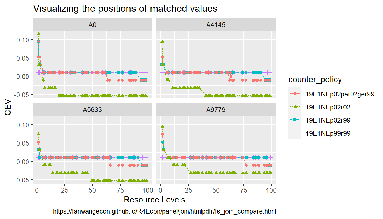

4.3.2 Within Panel Cross-time and Cross-group Statistics

Go back to fan’s REconTools research support package, R4Econ examples page, PkgTestR packaging guide, or Stat4Econ course page.

4.3.2.1 Comparing Three Countries over Time

Given three time series for three “countries”, we compute percentage change from initial year for each country, and compare relative values within each timer period versus one country.

First, we generate the core data inputs. We assume that the output here would be the data structure we face prior to generating the figures we are interested in. We use data from the attitude dataset, but re-interpret what the columns are. We work with data from three “countries” at the same time, which generalizes also to the two countries case.

# Load data, and treat index as "year"
# pretend data to be country-data
df_attitude <- as_tibble(attitude) %>%
  rowid_to_column(var = "year") %>% 
  select(year, rating, complaints, learning) %>% 
  rename(stats_usa = rating, 
         stats_canada = complaints, 
         stats_uk = learning)

# Wide to Long
df_attitude <- df_attitude %>%
  pivot_longer(cols = starts_with('stats_'),
               names_to = c('country'),
               names_pattern = paste0("stats_(.*)"),
               values_to = "rating")

# Print 
kable(df_attitude[1:10,]) %>% kable_styling_fc()

year	country	rating
1	usa	43
1	canada	51
1	uk	39
2	usa	63
2	canada	64
2	uk	54
3	usa	71
3	canada	70
3	uk	69
4	usa	61

Second, we generate additional data inputs. Specifically, we also generate ratios of values with respect to he “first” country, within each year.

# Sort and get list of countries
ar_countries_sorted <- df_attitude %>% 
  ungroup() %>% distinct(country) %>% arrange(country) %>% 
  pull(country)
st_ratio_var <- paste0('ratings_ratio_vs_country', ar_countries_sorted[1])

# Generate ratio over the first location
df_attitude <- df_attitude %>% 
  arrange(year, country) %>% group_by(year) %>% 
  mutate(!!sym(st_ratio_var) := rating/first(rating))
  
# Print 
kable(df_attitude[1:10,]) %>% kable_styling_fc()

year	country	rating	ratings_ratio_vs_countrycanada
1	canada	51	1.0000000
1	uk	39	0.7647059
1	usa	43	0.8431373
2	canada	64	1.0000000
2	uk	54	0.8437500
2	usa	63	0.9843750
3	canada	70	1.0000000
3	uk	69	0.9857143
3	usa	71	1.0142857
4	canada	63	1.0000000

Third, we now generate ratios of values with respect to the first year, within each country.

# Sort and get list of countries
ar_years_sorted <- df_attitude %>% 
  ungroup() %>% distinct(year) %>% arrange(year) %>% 
  pull(year)
st_ratio_var <- paste0('ratings_ratio_vs_year', ar_years_sorted[1])

# Generate ratio over the first location
df_attitude <- df_attitude %>% 
  arrange(country, year) %>% group_by(country) %>% 
  mutate(!!sym(st_ratio_var) := rating/first(rating))
  
# Print
# Within each country, we show the first 3 years 
kable(df_attitude %>% 
  group_by(country) %>% 
  slice_min(order_by = year, n = 3)
  ) %>% kable_styling_fc()

year	country	rating	ratings_ratio_vs_countrycanada	ratings_ratio_vs_year1
1	canada	51	1.0000000	1.000000
2	canada	64	1.0000000	1.254902
3	canada	70	1.0000000	1.372549
1	uk	39	0.7647059	1.000000
2	uk	54	0.8437500	1.384615
3	uk	69	0.9857143	1.769231
1	usa	43	0.8431373	1.000000
2	usa	63	0.9843750	1.465116
3	usa	71	1.0142857	1.651163

4.4 Join and Merge Files Together by Keys

4.4.1 Mesh Join

Go back to fan’s REconTools research support package, R4Econ examples page, PkgTestR packaging guide, or Stat4Econ course page.

4.4.1.1 Expand Multiple Rows with the Same Expansion

File A is at ID x Week x DayOfWeek level, file B is at ID x DayOfWeek x Product. Product is the product ID bought, could also store other info on product as additional variables. We want to create a file that is at ID x Week x DayOfweek x Product level.

The idea is that products bought made on Monday by household 1, for example are always the same, and file A records a “shopping-record”, which week, which day each household went shopping.

We do not store in file A what was bought because a particular household always buys the same thing on the same day of the week. We store data in A and B separately to save space since all products by the same household on the same day of week is always identical.

However, we need to join the two files together compute how many units of each product all households bought throughout some timeframe.

Step 1, construct File A, by fully messing ID, Week and Day of Week. In the simulated file below, household 1 shopped 3 times, twice on 3rd day of week, once on 2nd day of week, across two weeks. Household 2 shopped once, on the 3rd day of week.

# Mesh
ar_st_varnames <- c('hh','week','dayofweek')
ar_it_ids <- c(1,2)
ar_it_weeks <- c(1,2)
ar_it_daysofweek <- c(1,2,3)
df_idwkday_mesh <- tidyr::expand_grid(
  ar_it_ids, ar_it_weeks, ar_it_daysofweek) %>%
  rename_all(~c(ar_st_varnames))

# Randomly drop a subset of rows 
# Different subset of ID and Week for each DayOfWeek. 
it_M <- 4
set.seed(456)
df_idwkday_mesh <- df_idwkday_mesh[sample(dim(df_idwkday_mesh)[1], it_M, replace=FALSE),] %>% 
  arrange(!!!syms(ar_st_varnames))

# Display
st_caption <- "File A (ID x Week x DayOfWeek)"
kable(df_idwkday_mesh, caption=st_caption) %>% kable_styling_fc()

Table 4.7: File A (ID x Week x DayOfWeek)
hh	week	dayofweek
1	1	3
1	2	2
1	2	3
2	2	3

Step 2, construct File B. We have shopping list for the 1st household on shopping from 1st, 2nd, and 3rd days of a week. We have a shopping list for 2nd household only for shopping on the 1st and 2nd day.

# Generate day of week specific product file
ar_st_varnames <- c('hh', 'dayofweek', 'product')
ar_it_product <- c(10,11,12,13,14)
df_dayproduct_mesh <- tidyr::expand_grid(
  ar_it_ids, ar_it_daysofweek, ar_it_product) %>%
  rename_all(~c(ar_st_varnames))

# Make each day product list not identical
it_M <- 8
set.seed(123)
df_dayproduct_mesh <- df_dayproduct_mesh[sample(dim(df_dayproduct_mesh)[1], it_M, replace=FALSE),] %>% 
  arrange(!!!syms(ar_st_varnames))

# Display
st_caption <- "File B (ID x DayOfWeek x Product)"
kable(df_dayproduct_mesh, caption=st_caption) %>% kable_styling_fc()

Table 4.8: File B (ID x DayOfWeek x Product)
hh	dayofweek	product
1	1	12
1	2	14
1	3	10
1	3	13
1	3	14
2	1	12
2	1	13
2	2	11

Step 3. we combine files A and B together via dplyr::left_join.

Given the sample files we have constructed we have:

multiple items in shopping list for household 1 on day 3
no shopping list for household 2 on day 3
shopping list available on days that do not appear on shopping days tracking list

When we left_join, we do not include in combined file shopping list from days for households not in the tracking list. Note that from the output below, we achieved several things:

the day 3 shopping list for household 1 is merged in twice, to household’s trips on day 3 in both week 1 and 2, rows expanded because 3 items bought on each day
the day 2 shopping list for household 1 is merged in once, there are no row-expansion, since there was one item bought on this shopping list
the day 3 shopping list for household 2 is not merged in, since the shopping list does not exist, but the row remains.

# left join
df_left_join <- df_idwkday_mesh %>% 
  left_join(df_dayproduct_mesh, 
  by= c('hh'='hh', 'dayofweek'='dayofweek'))
# Display left-join
st_caption <- "File C, left-join (ID x Week x DayOfweek x Product)"
kable(df_left_join, caption=st_caption) %>% kable_styling_fc()

Table 4.9: File C, left-join (ID x Week x DayOfweek x Product)
hh	week	dayofweek	product
1	1	3	10
1	1	3	13
1	1	3	14
1	2	2	14
1	2	3	10
1	2	3	13
1	2	3	14
2	2	3	NA

Step 4, now, we also try dplyr::full_join. Note that the full-join result is not what we want, it added shopping list by household to the file, but these shopping lists were un-realized, since the households did not shop in any week on those days. So our desired result is achieved by dplyr::left_join.

# full join
df_full_join <- df_idwkday_mesh %>% 
  full_join(df_dayproduct_mesh, 
  by= c('hh'='hh', 'dayofweek'='dayofweek'))
# Display full-join
st_caption <- "File C, full-join (ID x Week x DayOfweek x Product)"
kable(df_full_join, caption=st_caption) %>% kable_styling_fc()

Table 4.10: File C, full-join (ID x Week x DayOfweek x Product)
hh	week	dayofweek	product
1	1	3	10
1	1	3	13
1	1	3	14
1	2	2	14
1	2	3	10
1	2	3	13
1	2	3	14
2	2	3	NA
1	NA	1	12
2	NA	1	12
2	NA	1	13
2	NA	2	11

hh	week	dayofweek	product
1	1	3	10
1	1	3	13
1	1	3	14
1	2	2	14
1	2	3	10
1	2	3	13
1	2	3	14
2	2	3	NA
1	NA	1	12
2	NA	1	12
2	NA	1	13
2	NA	2	11

hh	week	dayofweek	product
1	1	3	10
1	1	3	13
1	1	3	14
1	2	2	14
1	2	3	10
1	2	3	13
1	2	3	14
2	2	3	NA
1	NA	1	12
2	NA	1	12
2	NA	1	13
2	NA	2	11

hh	week	dayofweek	product
1	1	3	10
1	1	3	13
1	1	3	14
1	2	2	14
1	2	3	10
1	2	3	13
1	2	3	14
2	2	3	NA
1	NA	1	12
2	NA	1	12
2	NA	1	13
2	NA	2	11