Chapter 10 Tables and Graphs

10.1 R Base Plots

10.1.1 Plot Curve, Line and Points

Go back to fan’s REconTools research support package, R4Econ examples page, PkgTestR packaging guide, or Stat4Econ course page.

Work with the R plot function.

10.1.1.1 One Point, One Line and Two Curves

• r curve on top of plot
• r plot specify pch lty both scatter and line
• r legend outside

Jointly plot:

• 1 scatter plot
• 1 line plot
• 2 function curve plots

#######################################################
# First, Some common Labels:
#######################################################
# Labeling
st_title <- paste0('Scatter, Line and Curve Joint Ploting Example Using Base R\n',
                   'plot() + curve(): x*sin(x), cos(x), sin(x)*cos(x), sin(x)+tan(x)+cos(x)')
st_subtitle <- paste0('https://fanwangecon.github.io/',
                      'R4Econ/tabgraph/inout/htmlpdfr/fs_base_curve.html')
st_x_label <- 'x'
st_y_label <- 'f(x)'

#######################################################
# Second, Generate the Graphs Functions and data points:
#######################################################
# x only used for Point 1 and Line 1
x <- seq(-1*pi, 1*pi, length.out=25)
# Line (Point) 1: Generate X and Y
y1 <- x*sin(x)
st_point_1_y_legend <- 'x*sin(x)'
# Line 2: Line Plot
y2 <- cos(x)
st_line_2_y_legend <- 'cos(x)'
# Line 3: Function
fc_sin_cos_diff <- function(x) sin(x)*cos(x)
st_line_3_y_legend <- 'sin(x)*cos(x)'
# Line 4: Function
fc_sin_cos_tan <- function(x) sin(x) + cos(x) + tan(x)
st_line_4_y_legend <- 'sin(x) + tan(x) + cos(x)'

#######################################################
# Third, set:
# - point shape and size: *pch* and *cex*
# - line type and width: *lty* and *lwd*
#######################################################
# http://www.sthda.com/english/wiki/r-plot-pch-symbols-the-different-point-shapes-available-in-r
# http://www.sthda.com/english/wiki/line-types-in-r-lty
# for colors, see: https://fanwangecon.github.io/M4Econ/graph/tools/fs_color.html
st_point_1_blue <- rgb(57/255,106/255,177/255)
st_line_2_red <- rgb(204/255, 37/255, 41/255,)
st_line_3_black <- 'black'
st_line_4_purple <- 'orange'

# point type
st_point_1_pch <- 10
# point size
st_point_1_cex <- 2

# line type
st_line_2_lty <- 'dashed'
st_line_3_lty <- 'dotted'
st_line_4_lty <- 'dotdash'
# line width
st_line_2_lwd <- 3
st_line_3_lwd <- 2.5
st_line_4_lwd <- 3.5

#######################################################
# Fourth: Share xlim and ylim
#######################################################
ar_xlim = c(min(x), max(x))
ar_ylim = c(-3.5, 3.5)

#######################################################
# Fifth: the legend will be long, will place it to the right of figure,
#######################################################
par(new=FALSE, mar=c(5, 4, 4, 10))

#######################################################
# Sixth, the four objects and do not print yet:
#######################################################
# pdf(NULL)
# Graph Scatter 1
plot(x, y1, type="p",
     col = st_point_1_blue,
     pch = st_point_1_pch, cex = st_point_1_cex,
     xlim = ar_xlim, ylim = ar_ylim,
     panel.first = grid(),
     ylab = '', xlab = '', yaxt='n', xaxt='n', ann=FALSE)
pl_scatter_1 <- recordPlot()

# Graph Line 2
par(new=T)
plot(x, y2, type="l",
     col = st_line_2_red,
     lwd = st_line_2_lwd, lty = st_line_2_lty,
     xlim = ar_xlim, ylim = ar_ylim,
     ylab = '', xlab = '', yaxt='n', xaxt='n', ann=FALSE)
pl_12 <- recordPlot()

# Graph Curve 3
par(new=T)
curve(fc_sin_cos_diff,
      col = st_line_3_black,
      lwd = st_line_3_lwd, lty = st_line_3_lty,
      from = ar_xlim[1], to = ar_xlim[2], ylim = ar_ylim,
      ylab = '', xlab = '', yaxt='n', xaxt='n', ann=FALSE)
pl_123 <- recordPlot()

# Graph Curve 4
par(new=T)
curve(fc_sin_cos_tan,
      col = st_line_4_purple,
      lwd = st_line_4_lwd, lty = st_line_4_lty,
      from = ar_xlim[1], to = ar_xlim[2], ylim = ar_ylim,
      ylab = '', xlab = '', yaxt='n', xaxt='n', ann=FALSE)
pl_1234 <- recordPlot()
# invisible(dev.off())

#######################################################
# Seventh, Set Title and Legend and Plot Jointly
#######################################################
# CEX sizing Contorl Titling and Legend Sizes
fl_ces_fig_reg = 1
fl_ces_fig_small = 0.75

# R Legend
title(main = st_title, sub = st_subtitle, xlab = st_x_label, ylab = st_y_label,
      cex.lab=fl_ces_fig_reg,
      cex.main=fl_ces_fig_reg,
      cex.sub=fl_ces_fig_small)
axis(1, cex.axis=fl_ces_fig_reg)
axis(2, cex.axis=fl_ces_fig_reg)
grid()

# Legend sizing CEX
legend("topright",
       inset=c(-0.4,0),
       xpd=TRUE,
       c(st_point_1_y_legend, st_line_2_y_legend, st_line_3_y_legend, st_line_4_y_legend),
       col = c(st_point_1_blue, st_line_2_red, st_line_3_black, st_line_4_purple),
       pch = c(st_point_1_pch, NA, NA, NA),
       cex = fl_ces_fig_small,
       lty = c(NA, st_line_2_lty, st_line_3_lty, st_line_4_lty),
       lwd = c(NA, st_line_2_lwd, st_line_3_lwd,st_line_4_lwd),
       title = 'Legends',
       y.intersp=2)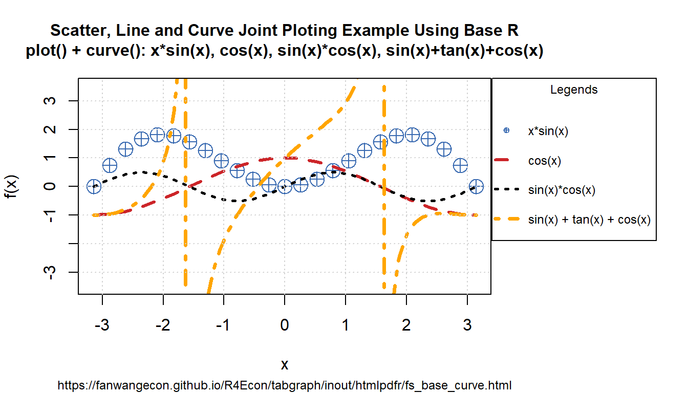

# record final plot
pl_1234_final <- recordPlot()

We used recordplot() earlier. So now we can print just the first two constructed plots.

#######################################################
# Eighth, Plot just the first two saved lines
#######################################################
# mar: margin, bottom, left, top, right
pl_12
# R Legend
par(new=T)
title(main = st_title, sub = st_subtitle, xlab = st_x_label, ylab = st_y_label,
      cex.lab = fl_ces_fig_reg,
      cex.main = fl_ces_fig_reg,
      cex.sub = fl_ces_fig_small)

# Legend sizing CEX
par(new=T)
legend("topright",
       inset=c(-0.4,0),
       xpd=TRUE,
       c(st_point_1_y_legend, st_line_2_y_legend),
       col = c(st_point_1_blue, st_line_2_red),
       pch = c(st_point_1_pch, NA),
       cex = fl_ces_fig_small,
       lty = c(NA, st_line_2_lty),
       lwd = c(NA, st_line_2_lwd),
       title = 'Legends',
       y.intersp=2)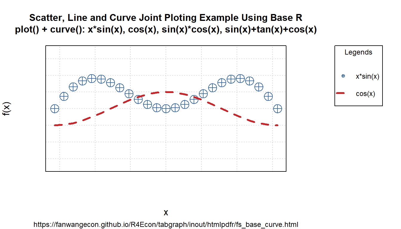

10.2 ggplot Line Related Plots

10.2.1 ggplot Line Plot Basics

Go back to fan’s REconTools research support package, R4Econ examples page, PkgTestR packaging guide, or Stat4Econ course page.

10.2.1.1 Two Time Series

Given three time series, we plot them jointly.

First, we construct a dataframe.

# Load data, and treat index as "year"
# pretend data to be country-data
df_attitude <- as_tibble(attitude) %>%
  rowid_to_column(var = "year") %>% 
  select(year, rating, complaints, learning) %>% 
  rename(stats_usa = rating, 
         stats_canada = complaints, 
         stats_uk = learning)

# Wide to Long
df_attitude <- df_attitude %>%
  pivot_longer(cols = starts_with('stats_'),
               names_to = c('country'),
               names_pattern = paste0("stats_(.*)"),
               values_to = "rating")

# Print 
kable(df_attitude[1:10,]) %>% kable_styling_fc()

year	country	rating
1	usa	43
1	canada	51
1	uk	39
2	usa	63
2	canada	64
2	uk	54
3	usa	71
3	canada	70
3	uk	69
4	usa	61

Second, we generate a basic visualizations with default values.

# basic chart with two lines
pl_lines_basic <- df_attitude %>% 
  ggplot(aes(x=year, y=rating, 
    color=country, linetype=country)) + 
  geom_line(size = 1) + 
  labs(x = paste0("Years"),
       y = paste0("Ratings"),
       title = paste(
        "Main Title for this Figure over",
        "Countries", sep=" "),
       subtitle = paste(
        "Subtitle for ratings changes across",
        "countries", sep=" "),
       caption = paste(
        "Caption for our figure here ",
        "This is the next line ", 
        "Another line", sep=""))
  
# print figure
print(pl_lines_basic)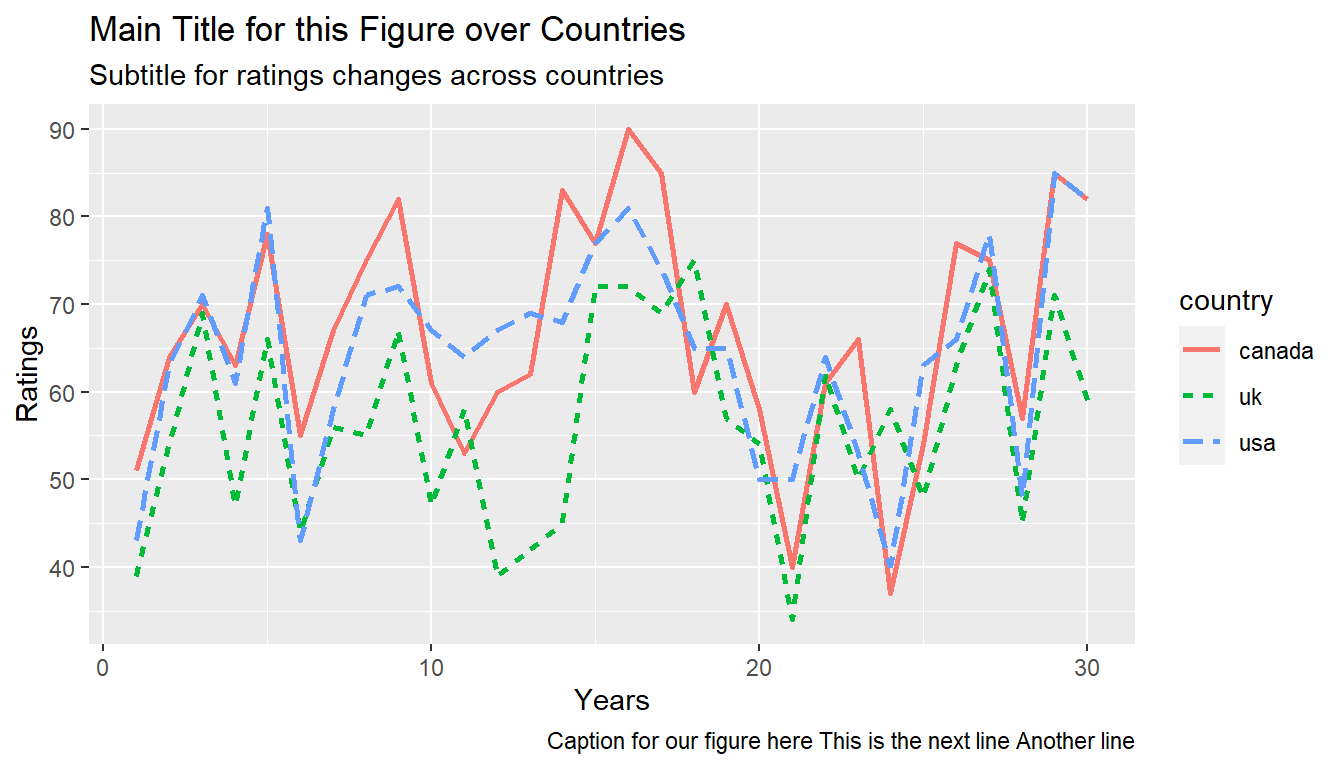

Third, we generate a more customized visualization with customized: (1) colors and shapes for lines; (2) x- and y-axis limits, labels, and breaks; (3) customized legend position.

# basic chart with two lines
pl_lines <- df_attitude %>% 
  ggplot(aes(x=year, y=rating, 
    color=country, linetype=country, shape=country)) + 
  geom_line(size=1)

# Titles
st_x = "Years"
st_y = "Ratings"
st_subtitle = "Ratings changes across countries"
pl_lines <- pl_lines +
  labs(
    x = st_x,
    y = st_y,
    subtitle = st_subtitle)
  
# Figure improvements
# set shapes and colors
ar_st_labels <- c(
  bquote("Canada"),
  bquote("UK"),
  bquote("USA"))

ar_st_colours <- c("#85ccff", "#026aa3", "red")
ar_st_linetypes <- c("solid", "dashed", "longdash")
pl_lines <- pl_lines +
  scale_colour_manual(values = ar_st_colours, labels = ar_st_labels) +
  scale_shape_discrete(labels = ar_st_labels) +
  scale_linetype_manual(values = ar_st_linetypes, labels = ar_st_labels)

# Axis
x_labels <- c("Yr 1990", "Year 2000", "Y 2010", "y-2015", "2020 (year)")
x_breaks <- c(0, 10, 20, 25, 30)
x_min <- 0
x_max <- 30

y_breaks <- seq(30, 90, length.out=6)
y_labels <- paste0('y=', y_breaks)
y_min <- 30
y_max <- 90

pl_lines <- pl_lines + 
  scale_x_continuous(
    labels = x_labels, breaks = x_breaks,
    limits = c(x_min, x_max)
  ) +
  theme(axis.text.x = element_text(
    # Adjust x-label angle
    angle = 45, 
    # Adjust x-label distance to x-axis (up vs down)
    hjust = 0.4, 
    # Adjust x-label left vs right wwith respect ot break point
    vjust = 0.5)) + 
  scale_y_continuous(
    labels = y_labels, breaks = y_breaks,
    limits = c(y_min, y_max)
  )

# print figure
print(pl_lines)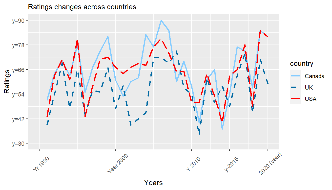

10.2.2 ggplot Line Advanced

Go back to fan’s REconTools research support package, R4Econ examples page, PkgTestR packaging guide, or Stat4Econ course page.

10.2.2.1 Continuous Y and X Variables, Three Categories, One is Subplot

Visualize one continuous variable, along the x-axis, given three categorical variables, with 12 combined categories \(3\times2\times2=12\):

• one as subplot (productivity type), 3 unique values
• one as line-color (gamma levels), 2 unique values
• one as line-type (GE vs PE), 2 unique values

The outcome is continuous CEV, generated for results with different productivity types (subplot), generated for PE vs GE (linetype), and at different parameter specifications (lower and higher gamma). X-axis is continuous. The graphs rely on this csv file cev_data.csv.

# Libraries
# library(tidyverse)

# Load in CSV
bl_save_img <- TRUE
spt_csv_root <- c("C:/Users/fan/R4Econ/tabgraph/ggline/_file/")
spt_img_root <- c("C:/Users/fan/R4Econ/tabgraph/ggline/_file/")
spn_cev_data <- paste0(spt_csv_root, "cev_data.csv")
spn_cev_graph <- paste0(spt_img_root, "cev_graph.png")
spn_cev_graph_eps <- paste0(spt_img_root, "cev_graph.eps")
df_cev_graph <- as_tibble(read.csv(spn_cev_data)) %>% select(-X)

# Dataset subsetting ------

# Line Patterns and Colors ------
# ar_st_age_group_leg_labels <- c("\nGE\n\u03B3=0.42\n", "\nGE\n\u03B3=0.56\n",
#                                 "\nPE\n\u03B3=0.42\n", "\nPE\n\u03B3=0.42\n")
ar_st_age_group_leg_labels <- c(
  bquote("GE," ~ gamma == .(0.42)),
  bquote("GE," ~ gamma == .(0.56)),
  bquote("PE," ~ gamma == .(0.42)),
  bquote("PE," ~ gamma == .(0.56))
)
ar_st_colours <- c("#85ccff", "#026aa3", "#85ccff", "#026aa3")
ar_st_linetypes <- c("solid", "solid", "longdash", "longdash")

# Labels and Other Strings -------
st_title <- ""
st_x <- "Wealth"
st_y <- "Welfare Gain (% CEV)"
st_subtitle <- paste0(
  "https://fanwangecon.github.io/",
  "R4Econ/tabgraph/ggline/htmlpdfr/fs_ggline_mgrp_ncts.html"
)

# ar_st_age_group_leg_labels <- c("C\u2013Optimal", "V\u2013Optimal")

prod_type_recode <- c(
  "Productivity Type\n(-1 sd)" = "8993",
  "Productivity Type\n(mean)" = "10189",
  "Productivity Type\n(+1 sd)" = "12244"
)

x_labels <- c("0", "200k", "400k", "600k", "800k")
x_breaks <- c(
  0,
  5,
  10,
  15,
  20
)
x_min <- 0
x_max <- 20

# y_labels <- c('-0.01',
#               '\u2191\u2191\nWelfare\nGain\n\nCEV=0\n\nWelfare\nLoss\n\u2193\u2193',
#               '+0.01', '+0.02', '+0.03', '+0.04','+0.05')
y_labels <- c(
  "-0.5 pp",
  "CEV=0",
  "+0.5 pp", "+1.0 pp", "+1.5 pp", "+2.0 pp", "+2.5 pp"
)
y_breaks <- c(-0.01, 0, 0.01, 0.02, 0.03, 0.04, 0.05)
y_min <- -0.011
y_max <- 0.051

# data change -------
df_cev_graph <- df_cev_graph %>%
  filter(across(counter_policy, ~ grepl("70|42", .))) %>%
  mutate(prod_type_lvl = as.factor(prod_type_lvl)) %>%
  mutate(prod_type_lvl = fct_recode(prod_type_lvl, !!!prod_type_recode))

# graph ------
pl_cev <- df_cev_graph %>%
  group_by(prod_type_st, cash_tt) %>%
  ggplot(aes(
    x = cash_tt, y = cev_lvl,
    colour = counter_policy, linetype = counter_policy, shape = counter_policy
  )) +
  facet_wrap(~prod_type_lvl, nrow = 1) +
  geom_smooth(method = "auto", se = FALSE, fullrange = FALSE, level = 0.95)

# labels
pl_cev <- pl_cev +
  labs(
    x = st_x,
    y = st_y,
    subtitle = st_subtitle
  )

# set shapes and colors
pl_cev <- pl_cev +
  scale_colour_manual(values = ar_st_colours, labels = ar_st_age_group_leg_labels) +
  scale_shape_discrete(labels = ar_st_age_group_leg_labels) +
  scale_linetype_manual(values = ar_st_linetypes, labels = ar_st_age_group_leg_labels) +
  scale_x_continuous(
    labels = x_labels, breaks = x_breaks,
    limits = c(x_min, x_max)
  ) +
  scale_y_continuous(
    labels = y_labels, breaks = y_breaks,
    limits = c(y_min, y_max)
  )

# Horizontal line
pl_cev <- pl_cev +
  geom_hline(yintercept = 0, linetype = "solid", colour = "black", size = 1)
# geom_hline(yintercept=0, linetype='dotted', colour="black", size=2)

# theme
pl_cev <- pl_cev +
  theme_bw() +
  theme(
    text = element_text(size = 10),
    legend.title = element_blank(),
    legend.position = c(0.16, 0.65),
    legend.background = element_rect(
      fill = "white",
      colour = "black",
      linetype = "solid"
    ),
    legend.key.width = unit(1.5, "cm")
  )

# Print Images to Screen -----
print(pl_cev)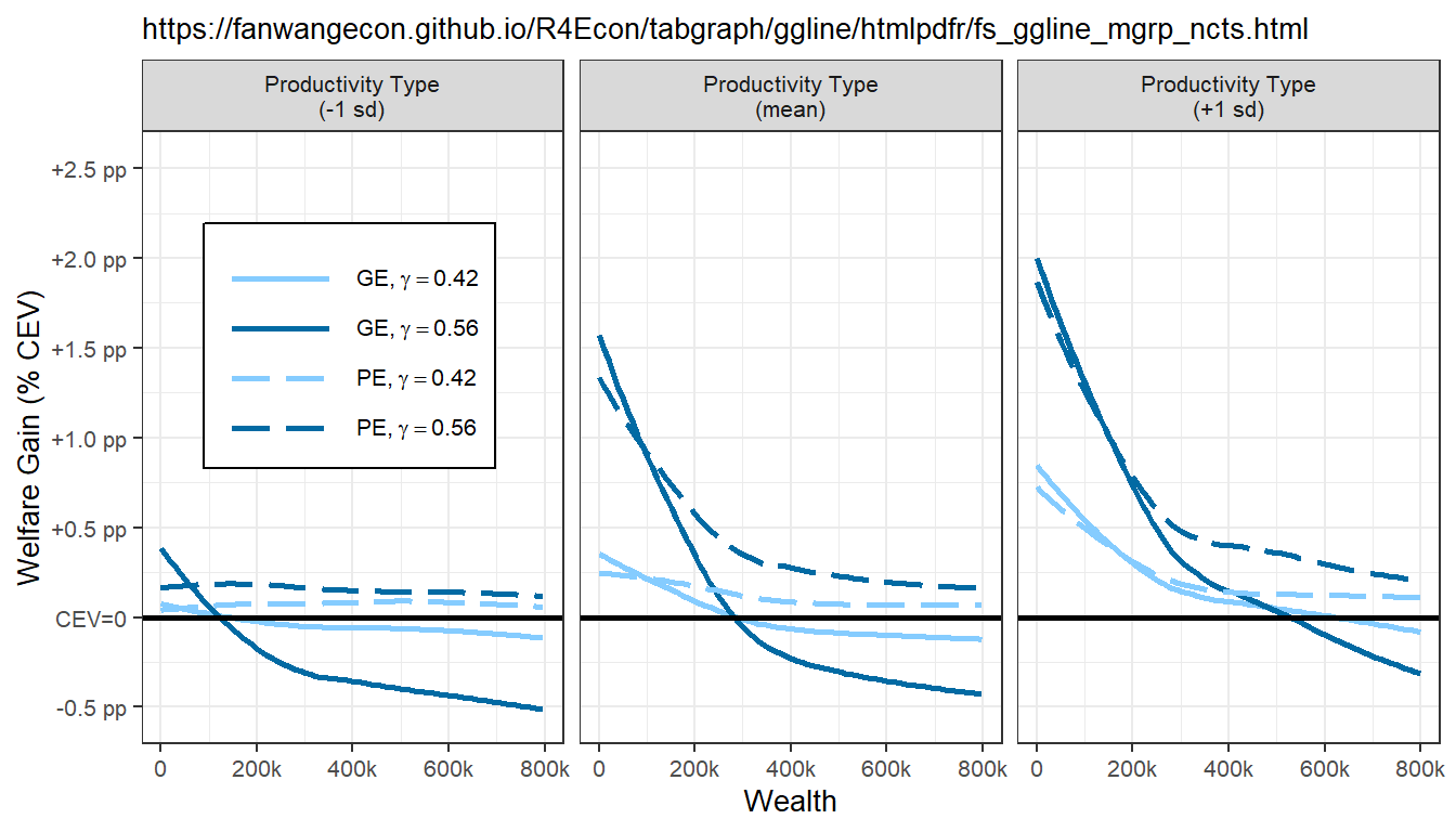

# Save Image Outputs -----
if (bl_save_img) {
  png(spn_cev_graph,
    width = 160,
    height = 105, units = "mm",
    res = 150, pointsize = 7
  )
  ggsave(
    spn_cev_graph_eps,
    plot = last_plot(),
    device = "eps",
    path = NULL,
    scale = 1,
    width = 200,
    height = 100,
    units = c("mm"),
    dpi = 150,
    limitsize = TRUE
  )
  print(pl_cev)
  dev.off()
}

## png 
##   2

10.2.2.2 Continuous Y and X Variables, Two Categories, One is Subplot

In contrast to the first line plot, in this second example, we use both varying line color as well as line shape and scatter type to distinguish categories of one categorical variable. Visualize one continuous variable, along the x-axis, given three categorical variables, with 10 combined categories \(2\times5=10\):

• one as subplot (GE vs PE), 2 unique values
• one with line-color, line-color and scatter shape joint variation (counterfactual type), 5 unique values

The outcome is change in male and female labor participation gaps, generated under partial and general equilibrium (subplot), generated for different counterfactual policies (linetype). X-axis is calendar year. Features:

• Calendar year as x-axis
• Line + scatter with varying line patterns and scatter shapes
• Scatter shapes
• Show five lines together, with 2 lines stand out more, and 4 lines overall different than 1
• Legend box area with longer legend text, transparent and no border

For data processing, converts all possible numerical variables to numeric.

# Load in CSV
bl_save_img <- TRUE
spt_csv_root <- c("C:/Users/fan/R4Econ/tabgraph/ggline/_file/")
spt_img_root <- spt_csv_root
spn_flfp_sklocc_data <- paste0(spt_csv_root, "flfp_data.csv")
spn_flfp_sklocc_graph <- paste0(spt_img_root, "flfp_sam2fshr_graph.png")
spn_flfp_sklocc_graph_eps <- paste0(spt_img_root, "flfp_sam2fshr_graph.eps")

# Load data
# Convert all convertable numeric columns from string to numeric
# https://stackoverflow.com/a/49054046/8280804
is_all_numeric <- function(x) {
  !any(is.na(suppressWarnings(as.numeric(na.omit(x))))) & is.character(x)
}
df_flfp <- as_tibble(read.csv(spn_flfp_sklocc_data)) %>%
  mutate_if(is_all_numeric, as.numeric) %>%
  filter(year <= 2014)

# Dataset subsetting ------

# Line Patterns and Colors ------
ctr_var_recode <- c(
  "No change" = "1",
  "Married" = "31",
  "Children < 5" = "32",
  "Appliance" = "33",
  "WBL Index" = "34"
)

# https://www.rgbtohex.net/
ar_st_colours <- c("#262626", "#FFC001", "#ED8137", "#4472C4", "#3E9651")
# http://www.sthda.com/english/wiki/ggplot2-line-types-how-to-change-line-types-of-a-graph-in-r-software
ar_st_linetypes <- c("dashed", "solid", "solid", "solid", "solid")
# http://sape.inf.usi.ch/quick-reference/ggplot2/shape
# 32 is invisible shape
ar_it_shapes <- c(32, 5, 17, 15, 1)

# Labels and Other Strings -------
st_title <- ""
st_x <- "Years"
st_y <- "Change in Aggregate (Male - Female) Participation Shares"
st_subtitle <- paste0(
  "https://fanwangecon.github.io/",
  "R4Econ/tabgraph/ggline/htmlpdfr/fs_ggline_mgrp_ncts.html"
)

# ge_pe_recode <- c(
#   "General Equilibrium\n(Adjust Wages)" = "GE",
#   "Partial Equilibrium\n(Wage as Observed)" = "PE"
# )
ge_pe_recode <- c(
  "General Equilibrium" = "GE",
  "Partial Equilibrium" = "PE"
)
# x.breaks <- c(1989, seq(1992, 2004, by = 2), 2005, seq(2008, 2014, by = 2))
# x.labels <- paste(x.breaks[1:13])
x.breaks <- seq(1989, 2014, by = 5)
x.labels <- paste(x.breaks[1:6])
x.min <- 1989
x.max <- 2014

y.breaks <- round(seq(-0.30, 0.05, by = 0.05), 2)
y.labels <- paste0(paste(y.breaks[1:length(y.breaks)] * 100), "%")

y.min <- -0.26
y.max <- 0.01

# data change -------
df_flfp_sklocc_graph <- df_flfp %>%
  filter(ctr_var_idx %in% c(1, 31, 32, 33, 34) & category == "C001") %>%
  mutate(
    ge_pe = as.factor(ge_pe),
    ctr_var_idx = as.factor(ctr_var_idx)
  ) %>%
  mutate(ge_pe = fct_recode(ge_pe, !!!ge_pe_recode)) %>%
  mutate(ctr_var_idx = fct_recode(ctr_var_idx, !!!ctr_var_recode)) %>%
  select(year, ctr_var_idx, ge_pe, part_yeargender_shr_m2f_dfv1st)

# graph ------
pl_flfp_agg <- df_flfp_sklocc_graph %>%
  ggplot(aes(
    x = year, y = part_yeargender_shr_m2f_dfv1st,
    colour = ctr_var_idx, linetype = ctr_var_idx, shape = ctr_var_idx
  )) +
  facet_wrap(~ge_pe, nrow = 1) +
  geom_line() +
  geom_point()

# labels
pl_flfp_agg <- pl_flfp_agg +
  labs(
    x = st_x,
    y = st_y
  )
# subtitle = st_subtitle

# set shapes and colors
# scale_colour_manual(values = ar_st_colours, labels = ctr_var_recode) +
# scale_shape_manual(values=ar_it_shapes, labels = ctr_var_recode) +
# scale_linetype_manual(values = ar_st_linetypes, labels = ctr_var_recode) +
pl_flfp_agg <- pl_flfp_agg +
  scale_colour_manual(values = ar_st_colours) +
  scale_shape_manual(values = ar_it_shapes) +
  scale_linetype_manual(values = ar_st_linetypes) +
  scale_x_continuous(
    labels = x.labels, breaks = x.breaks,
    limits = c(x.min, x.max)
  ) +
  scale_y_continuous(
    labels = y.labels, breaks = y.breaks,
    limits = c(y.min, y.max)
  )

# Horizontal line
pl_flfp_agg <- pl_flfp_agg +
  geom_hline(yintercept = 0, linetype = "solid", colour = "black", size = 1)
# geom_hline(yintercept=0, linetype='dotted', colour="black", size=2)

# theme
pl_flfp_agg <- pl_flfp_agg +
  theme_bw() +
  theme(
    text = element_text(size = 11),
    legend.title = element_text(size = 10),
    legend.margin = margin(c(0.1, 0.1, 0.1, 0.1), unit = "cm"),
    legend.position = c(0.10, 0.27),
    legend.background = element_rect(
      fill = "white",
      colour = "black",
      linetype = "solid"
    ),
    legend.key.width = unit(1.0, "cm"),
    axis.title.y = element_text(size = 10)
  ) +
  guides(
    color = guide_legend(title = "Set to 1989 Level:"),
    linetype = guide_legend(title = "Set to 1989 Level:"),
    shape = guide_legend(title = "Set to 1989 Level:")
  )

# Print Images to Screen 
print(pl_flfp_agg)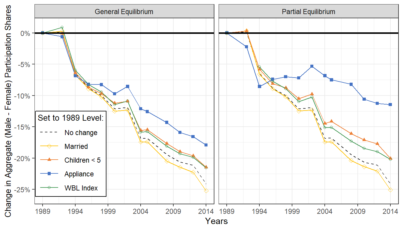

# Save Image Outputs -----
if (bl_save_img) {
  png(spn_flfp_sklocc_graph,
    width = 200,
    height = 100, units = "mm",
    res = 150, pointsize = 7
  )
  ggsave(
    spn_flfp_sklocc_graph_eps,
    plot = last_plot(),
    device = "eps",
    path = NULL,
    scale = 1,
    width = 200,
    height = 100,
    units = c("mm"),
    dpi = 150,
    limitsize = TRUE
  )
  print(pl_flfp_agg)
  dev.off()
}

## png 
##   2

10.2.2.3 Continuous Y and X Variables, Four Categories, Three for Subplot

In contrast to the line plot above, in this third example, we have three categorical variables that will be visualized via plots and subplots. We have four categoricalv variables overall, for the fourth categorical variable, as in the second example, we continue to use both varying line color as well as line shape and scatter type to distinguish categories of this fourth categorical variable. Visualize one continuous variable, along the x-axis, given four categorical variables, with 60 combined categories \(3\times2\times2\times3=36\):

• one as plot, generate three different plots, 3 unique values, achieved by saving a function and running the function three times with variable conditioning.
• one as facet_grid row group, 2 unique values.
• one as facet_grid column group, 2 unique values.
• one with line-color, line-color and scatter shape joint variation (counterfactual type), 3 unique values

Following the example above, continue to analyze female labor participation. Generated under partial and general equilibrium (subplot), and skill and occupational groups. , generated for different counterfactual policies (linetype). X-axis is calendar year.

Features:

• facet_grid: Multiple rows and columns for faceting, row and column labels
• No spacing for empty title line
• Graph as function with simple variable and parameter adjustment
• No minor grid
• Do not show ylabel.

First define the graphing function:

# The graphing function with limited parameter options.
ff_grhlfp_gepeedu_byocc <-
  function(bl_save_img = TRUE,
           st_occ = "Manual",
           y_breaks = round(seq(0.08, 0.18, by = 0.02), 2),
           y_min = 0.08,
           y_max = 0.19,
           ar_leg_position = c(0.29, 0.50),
           it_width = 160, it_height = 105,
           st_subtitle = paste0(
             "https://fanwangecon.github.io/",
             "R4Econ/tabgraph/ggline/htmlpdfr/fs_ggline_mgrp_ncts.html"
           )) {

    # Load in CSV
    spt_csv_root <- c("C:/Users/fan/R4Econ/tabgraph/ggline/_file/")
    spt_img_root <- spt_csv_root
    spn_flfp_sklocc_data <- paste0(spt_csv_root, "flfp_data.csv")
    spn_flfp_sklocc_graph <- paste0(
      spt_img_root,
      paste0("flfp_gepe_colhigh_", tolower(st_occ), "_graph.png")
    )
    spn_flfp_sklocc_graph_eps <- paste0(
      spt_img_root,
      paste0("flfp_gepe_colhigh_", tolower(st_occ), "_graph.eps")
    )

    # Load data
    # Convert all convertable numeric columns from string to numeric
    # https://stackoverflow.com/a/49054046/8280804
    is_all_numeric <- function(x) {
      !any(is.na(suppressWarnings(as.numeric(na.omit(x))))) & is.character(x)
    }
    df_flfp <- as_tibble(read.csv(spn_flfp_sklocc_data)) %>%
      mutate_if(is_all_numeric, as.numeric) %>%
      filter(year <= 2014)

    # Dataset subsetting ------

    # Line Patterns and Colors ------
    ctr_var_recode <- c(
      "Prediction no Counterfactual" = "1",
      "Married at 1989 Levels" = "31",
      "Children < 5 at 1989 Levels" = "32",
      "Appliance at 1989 Levels" = "33",
      "WBL Index at 1989 Levels" = "34"
    )

    # https://www.rgbtohex.net/
    # ar_st_colours <- c("#262626", "#FFC001", "#ED8137", "#4472C4", "#3E9651")
    ar_st_colours <- c("#262626", "#ED8137", "#4472C4")
    # http://www.sthda.com/english/wiki/ggplot2-line-types-how-to-change-line-types-of-a-graph-in-r-software
    ar_st_linetypes <- c("dashed", "solid", "solid")
    # http://sape.inf.usi.ch/quick-reference/ggplot2/shape
    # 32 is invisible shape
    # ar_it_shapes <- c(32, 5, 17, 15, 1)
    ar_it_shapes <- c(32, 17, 15)

    # Labels and Other Strings -------
    st_x <- "Years"
    st_y <- paste0("Female ", st_occ, " Occupation Participation Shares")

    # ge_pe_recode <- c(
    #   "General Equilibrium\n(Adjust Wages)" = "GE",
    #   "Partial Equilibrium\n(Wage as Observed)" = "PE"
    # )
    ge_pe_recode <- c(
      "General Equilibrium" = "GE",
      "Partial Equilibrium" = "PE"
    )
    # ge_pe_recode <- c(
    #   "GE" = "GE",
    #   "PE" = "PE"
    # )

    skilled_unskilled_recode <- c(
      "College Women" = "skilled",
      "Secondary Women" = "unskilled"
    )

    # x_breaks <- seq(1989, 2014, by = 5)
    x_breaks <- c(1990, 1995, 2000, 2005, 2010)
    x_labels <- paste(x_breaks[1:length(x_breaks)])
    x_min <- 1989
    x_max <- 2014

    # y_breaks <- round(seq(0.08, 0.18, by = 0.02), 2)
    y_labels <- paste0(paste(y_breaks[1:length(y_breaks)] * 100), "%")

    # y_min <- 0.08
    # y_max <- 0.19

    # data change -------
    df_flfp_sklocc_graph <- df_flfp %>%
      filter(ctr_var_idx %in% c(1, 32, 33) &
        gender == "Female" &
        occupation %in% c(st_occ)) %>%
      mutate(
        ge_pe = as.factor(ge_pe),
        ctr_var_idx = as.factor(ctr_var_idx)
      ) %>%
      mutate(
        ge_pe = fct_recode(ge_pe, !!!ge_pe_recode),
        skill = fct_recode(skill, !!!skilled_unskilled_recode),
        ctr_var_idx = fct_recode(ctr_var_idx, !!!ctr_var_recode)
      ) %>%
      select(year, skill, occupation, ctr_var_idx, ge_pe, genskl_part_share)

    # graph ------
    pl_flfp_sklocc <- df_flfp_sklocc_graph %>%
      ggplot(aes(
        x = year, y = genskl_part_share,
        colour = ctr_var_idx, linetype = ctr_var_idx, shape = ctr_var_idx
      )) +
      facet_grid(skill ~ ge_pe) +
      geom_line() +
      geom_point()

    # labels
    if (st_subtitle == "") {
      pl_flfp_sklocc <- pl_flfp_sklocc +
        labs(
          x = st_x,
          y = st_y
        )
    } else {
      pl_flfp_sklocc <- pl_flfp_sklocc +
        labs(
          x = st_x,
          y = st_y,
          subtitle = st_subtitle
        )
    }

    # set shapes and colors
    pl_flfp_sklocc <- pl_flfp_sklocc +
      scale_colour_manual(values = ar_st_colours) +
      scale_shape_manual(values = ar_it_shapes) +
      scale_linetype_manual(values = ar_st_linetypes) +
      scale_x_continuous(
        labels = x_labels, breaks = x_breaks,
        limits = c(x_min, x_max)
      ) +
      scale_y_continuous(
        labels = y_labels, breaks = y_breaks,
        limits = c(y_min, y_max)
      )

    # theme
    pl_flfp_sklocc <- pl_flfp_sklocc +
      theme_bw() +
      theme(
        text = element_text(size = 11),
        panel.grid.minor = element_blank(),
        legend.title = element_blank(),
        legend.position = ar_leg_position,
        legend.margin = margin(c(0.1, 0.1, 0.1, 0.1), unit = "cm"),
        legend.background = element_rect(
          fill = "white",
          colour = "black",
          linetype = "solid"
        ),
        legend.key.width = unit(1.0, "cm"),
        axis.text.x = element_text(angle = 45, vjust = 0.1, hjust = 0.1)
        # axis.text.y = element_text(angle = 90, hjust = 0.4)
      )
    # element_text(angle = 90, hjust = 0.4)
    # axis.title.y = element_blank(), # no y-label

    # Save Image Outputs -----
    if (bl_save_img) {
      ggsave(
        spn_flfp_sklocc_graph,
        plot = last_plot(),
        device = "png",
        path = NULL,
        scale = 1,
        width = it_width,
        height = it_height,
        units = c("mm"),
        dpi = 150,
        limitsize = TRUE
      )
      ggsave(
        spn_flfp_sklocc_graph_eps,
        plot = last_plot(),
        device = "eps",
        path = NULL,
        scale = 1,
        width = it_width,
        height = it_height,
        units = c("mm"),
        dpi = 150,
        limitsize = TRUE
      )
       # dev.off()
    }

    return(pl_flfp_sklocc)
  }

Second, run the function, for Manual, Routine and Analytical Works Separately.

it_width <- 100
it_height <- 100
st_subtitle <- paste0(
  "https://fanwangecon.github.io/",
  "R4Econ/tabgraph/ggline/htmlpdfr/fs_ggline_mgrp_ncts.html"
)
st_subtitle <- ""
# Manual,
pl_flfp_sklocc_manual <- ff_grhlfp_gepeedu_byocc(
  bl_save_img = TRUE,
  st_occ = "Manual",
  y_breaks = round(seq(0.00, 0.25, by = 0.05), 2),
  y_min = 0.00, y_max = 0.25,
  ar_leg_position = c(0.50, 0.80),
  it_width = it_width, it_height = it_height,
  st_subtitle = st_subtitle
)
print(pl_flfp_sklocc_manual)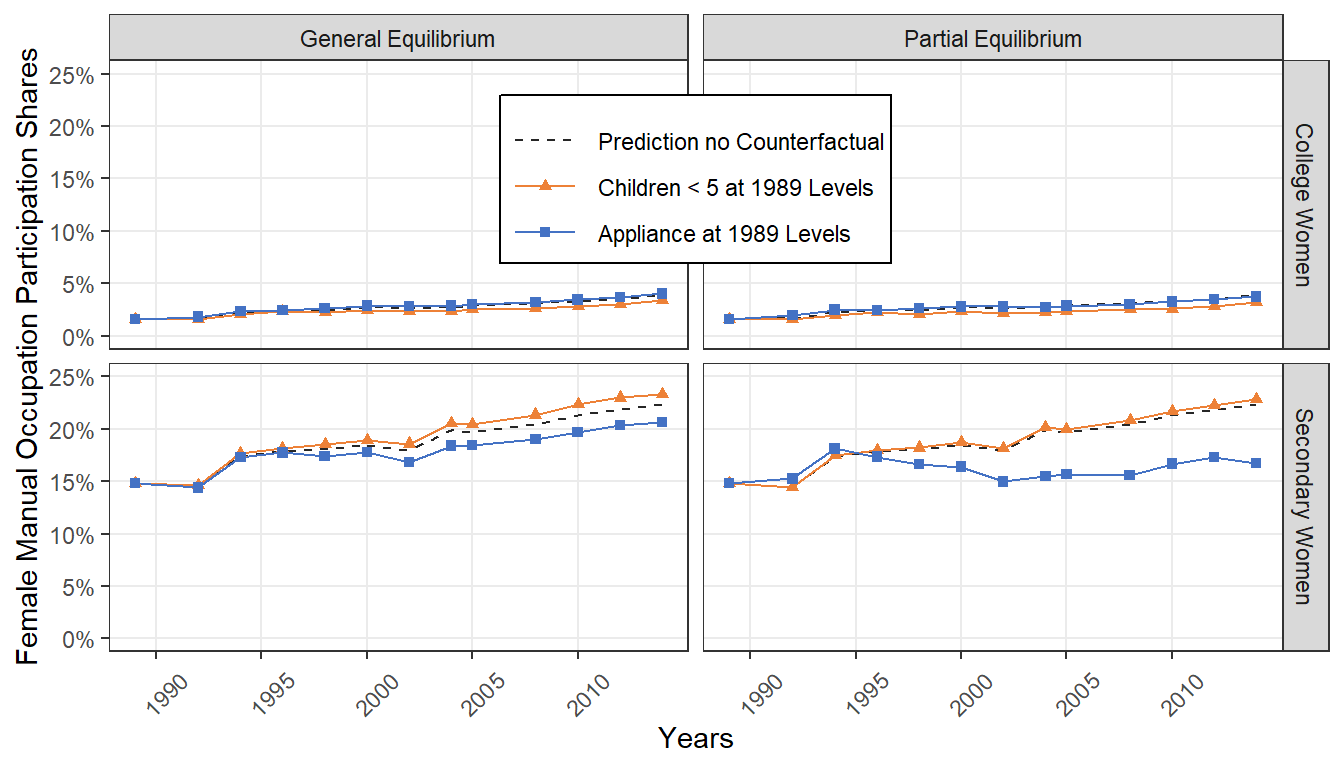

# Routine
pl_flfp_sklocc_routine <- ff_grhlfp_gepeedu_byocc(
  bl_save_img = TRUE,
  st_occ = "Routine",
  y_breaks = round(seq(0.08, 0.18, by = 0.02), 2),
  y_min = 0.08, y_max = 0.19,
  ar_leg_position = "none",
  it_width = it_width, it_height = it_height,
  st_subtitle = st_subtitle
)
print(pl_flfp_sklocc_routine)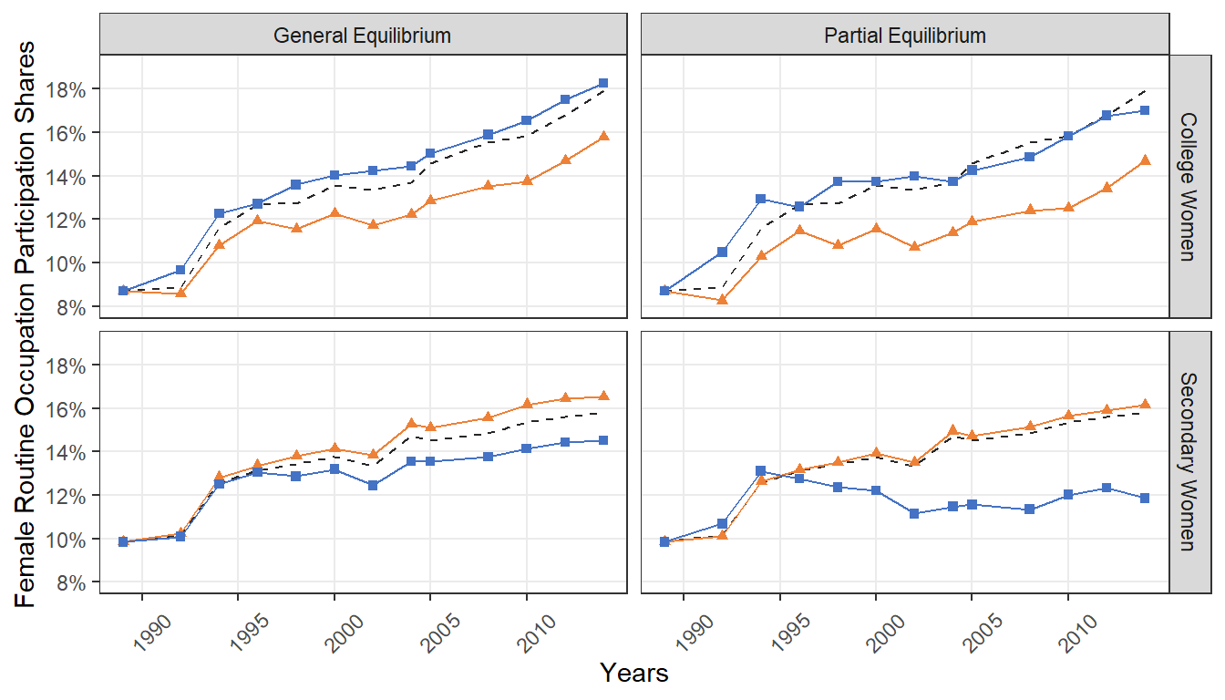

# Analytical
pl_flfp_sklocc_analytical <- ff_grhlfp_gepeedu_byocc(
  bl_save_img = TRUE,
  st_occ = "Analytical",
  y_breaks = round(seq(0.10, 0.60, by = 0.10), 2),
  y_min = 0.05, y_max = 0.60,
  ar_leg_position = "none",
  it_width = it_width, it_height = it_height,
  st_subtitle = st_subtitle
)
print(pl_flfp_sklocc_analytical)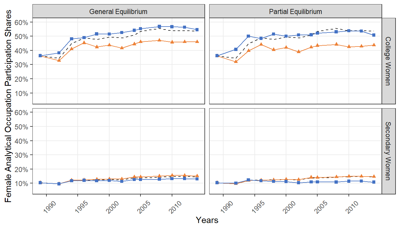

10.2.3 Time-series Plots with Shaded Areas

Go back to fan’s REconTools research support package, R4Econ examples page, PkgTestR packaging guide, or Stat4Econ course page.

10.2.3.1 Single Time-series with Single Type of Shade

We will construct three country-specific fake GDP time-series (converted from the attitude dataset). Then we will randomly select a subset of months and shade these months. This will generate a “recession” plot, where recession periods are shaded.

One of the assumption will be that we have data at discrete intervals, and the shaded areas will take mid-points.

First, we repeat the basic time-series data construction found in R4Econ.fs_ggline_basic.

# Load data, and treat index as "year", pretend data to be country-data
df_gdp <- as_tibble(attitude) %>%
    rowid_to_column(var = "year") %>%
    select(year, rating, complaints, learning) %>%
    rename(stats_usa = rating, stats_uk = learning) %>%
    pivot_longer(
        cols = starts_with("stats_"),
        names_to = c("country"),
        names_pattern = paste0("stats_(.*)"),
        values_to = "gdp"
    )

# Print
kable(df_gdp[1:10, ]) %>% kable_styling_fc()

year	complaints	country	gdp
1	51	usa	43
1	51	uk	39
2	64	usa	63
2	64	uk	54
3	70	usa	71
3	70	uk	69
4	63	usa	61
4	63	uk	47
5	78	usa	81
5	78	uk	66

Second, we select a subset of period to shade. We generate a random subset of non-overlapping consecutive numbers following what is outlined in R4Econ.fs_ary_generate.

# Number of random starting index
it_start_idx <- min(df_gdp$year)
it_end_idx <- max(df_gdp$year)
it_startdraws_max <- 6
it_duramax <- 2
it_backward_win <- 0.3
it_forward_win <- 0.3

# Random seed
set.seed(1234)
# Draw random index between min and max
ar_it_start_idx <- sort(sample(
    seq(it_start_idx, it_end_idx),
    it_startdraws_max,
    replace = FALSE
))
# Draw random durations, replace = TRUE because can repeat
ar_it_duration <- sample(it_duramax, it_startdraws_max, replace = TRUE)

# Check space between starts
ar_it_startgap <- diff(ar_it_start_idx)
ar_it_dura_lenm1 <- ar_it_duration[1:(length(ar_it_duration) - 1)]
# Adjust durations
ar_it_dura_bd <- pmin(ar_it_startgap - 2, ar_it_dura_lenm1)
ar_it_duration[1:(length(ar_it_duration) - 1)] <- ar_it_dura_bd

# Drop consecutive starts
ar_bl_dura_nonneg <- which(ar_it_duration >= 0)
ar_it_start_idx <- ar_it_start_idx[ar_bl_dura_nonneg]
ar_it_duration <- ar_it_duration[ar_bl_dura_nonneg]

# Print
print(glue::glue(
    "random starts + duration: ",
    "{ar_it_start_idx} + {ar_it_duration}"
))

## random starts + duration: 5 + 1
## random starts + duration: 12 + 1
## random starts + duration: 16 + 1
## random starts + duration: 22 + 2
## random starts + duration: 26 + 0
## random starts + duration: 28 + 2

Third, convert integers to half-point mid-distance, unless exceed lower or upper bounds, and build start and end points. We also construct back and forward window around

# Offset by half of an integer
ar_fl_start_time <- ar_it_start_idx - 0.5
ar_fl_end_time <- ar_it_start_idx + ar_it_duration + 0.5

# Bound by min and max
ar_fl_end_time <- pmin(ar_fl_end_time, it_end_idx)
ar_fl_start_time <- pmax(ar_fl_start_time, it_start_idx)

# Backward window
ar_fl_end_time_win_backward <- ar_fl_start_time
ar_fl_start_time_win_backward <- pmax(
    ar_fl_start_time - it_backward_win, it_start_idx
)

# Forward window
ar_fl_end_time_win_forward <- pmin(
    ar_fl_end_time + it_forward_win, it_end_idx
)
ar_fl_start_time_win_forward <- ar_fl_end_time

# Print
print(glue::glue(
    "random start-time vs end-time: ",
    "{ar_fl_start_time} + {ar_fl_end_time}"
))

## random start-time vs end-time: 4.5 + 6.5
## random start-time vs end-time: 11.5 + 13.5
## random start-time vs end-time: 15.5 + 17.5
## random start-time vs end-time: 21.5 + 24.5
## random start-time vs end-time: 25.5 + 26.5
## random start-time vs end-time: 27.5 + 30

Fourth, we construct a dataframe with variables as start and end of each non-overlapping recessions. We have a main window, and a lower and upper window bounds as well.

# Variable names
# w1 = backward, w2 = main, w3 = forward, use w1, w2, w3 to facilate legend fill sorting
ar_st_varnames <- c(
    "recess_id",
    "year_start_w2", "year_end_w2",
    "year_start_w1", "year_end_w1",
    "year_start_w3", "year_end_w3"
)

# Recession index file
df_recession <- as_tibble(cbind(
    ar_fl_start_time, ar_fl_end_time,
    ar_fl_start_time_win_backward, ar_fl_end_time_win_backward,
    ar_fl_start_time_win_forward, ar_fl_end_time_win_forward
)) %>%
    rowid_to_column() %>%
    rename_all(~ c(ar_st_varnames))

# Reshape from Wide to Long
df_recession <- df_recession %>%
    pivot_longer(
        cols = starts_with("year"),
        names_to = c("time", "window"),
        names_pattern = "year_(.*)_(.*)",
        values_to = "year"
    ) %>%
    pivot_wider(
        id_cols = c("recess_id", "window"),
        names_from = time,
        names_prefix = "year_",
        values_from = year
    )

Fifth, visualize time-series with shaded areas for “recessions”. Note that we are considering here “recessions” that are not country-specific.

# basic chart with two lines
pl_lines_basic <- ggplot() +
    geom_line(data = df_gdp, aes(
        x = year, y = gdp,
        color = country, linetype = country
    ), size = 1) +
    geom_rect(data = df_recession %>%
        filter(window == "w2"), aes(
        xmin = year_start, xmax = year_end,
        ymin = -Inf, ymax = Inf
    ), alpha = 0.6, fill = "gray") +
    labs(
        x = paste0("Years"),
        y = paste0("Ratings"),
        title = paste(
            "Main Title for this Figure over Countries (Shaded Recessions)",
            sep = " "
        ),
        subtitle = paste(
            "Subtitle for ratings changes across",
            "countries",
            sep = " "
        ),
        caption = paste(
            "Caption for our figure here ",
            "This is the next line ",
            "Another line",
            sep = ""
        )
    ) +
    theme_light() +
    facet_wrap(~country, ncol = 1)

# print figure
print(pl_lines_basic)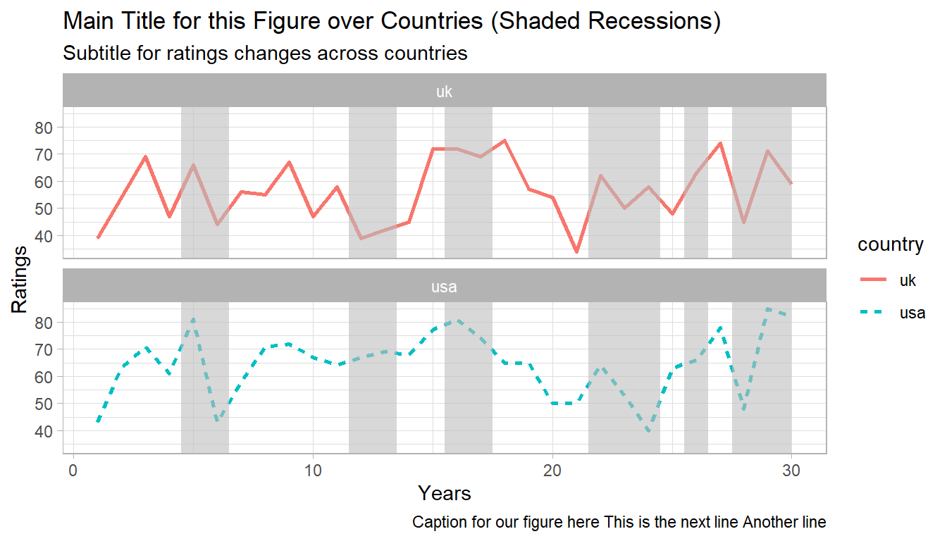

Sixth, we generate a more customized visualization with customized: (1) colors and shapes for lines as well as for windows; (2) x- and y-axis limits, labels, and breaks; (3) customized legend position.

# Window color
st_win_leg_title <- "Window"
st_win_color <- "gray"
st_win_label <- "Recession"
# basic chart with two lines
pl_lines <- ggplot() +
    geom_line(data = df_gdp, aes(
        x = year, y = gdp,
        color = country, linetype = country
    ), size = 1) +
    geom_rect(data = df_recession %>%
        filter(window == "w2"), aes(
        xmin = year_start, xmax = year_end,
        ymin = -Inf, ymax = Inf,
        fill = st_win_color
    ), alpha = 0.6) +
    theme_light()

# Titles
st_x <- "Years"
st_y <- "GDP"
st_subtitle <- "GDP changes across countries (shaded recessions)"
pl_lines <- pl_lines +
    labs(
        x = st_x,
        y = st_y,
        subtitle = st_subtitle
    )

# Figure improvements
# set shapes and colors
st_line_leg_title <- "Country"
ar_st_labels <- c(
    bquote("UK"),
    bquote("USA")
)

ar_st_colours <- c("#026aa3", "red")
ar_st_linetypes <- c("solid", "longdash")
pl_lines <- pl_lines +
    scale_colour_manual(values = ar_st_colours, labels = ar_st_labels) +
    scale_shape_discrete(labels = ar_st_labels) +
    scale_linetype_manual(values = ar_st_linetypes, labels = ar_st_labels) +
    scale_fill_manual(values = c(st_win_color), labels = c(st_win_label)) +
    labs(
        fill = st_win_leg_title,
        colour = st_line_leg_title, linetype = st_line_leg_title
    ) +
    theme(legend.key.width = unit(2.5, "line"))

# Axis
x_breaks <- seq(1, 30, length.out = 30)
x_labels <- paste0("Year ", x_breaks + 1990)

x_min <- 1
x_max <- 30

y_breaks <- seq(30, 90, length.out = 6)
y_labels <- paste0("y=", y_breaks)
y_min <- 30
y_max <- 90

pl_lines <- pl_lines +
    scale_x_continuous(
        labels = x_labels, breaks = x_breaks,
        limits = c(x_min, x_max)
    ) +
    theme(axis.text.x = element_text(
        # Adjust x-label angle
        angle = 90,
        # Adjust x-label distance to x-axis (up vs down)
        hjust = 0.4,
        # Adjust x-label left vs right wwith respect ot break point
        vjust = 0.5
    )) +
    scale_y_continuous(
        labels = y_labels, breaks = y_breaks,
        limits = c(y_min, y_max)
    )

# print figure
print(pl_lines)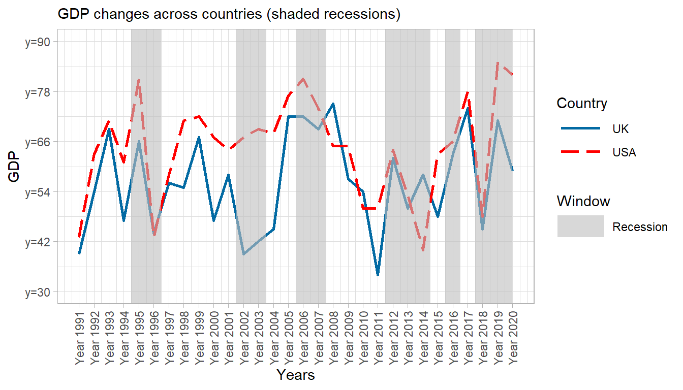

Finally, we generate a figure with three fill colors for the three windows, main, backward, and forward windows. We reuse various parameters used in the prior block.

# Window color
st_win_leg_title <- "Window"
# basic chart with two lines
pl_lines <- ggplot() +
    geom_line(data = df_gdp, aes(
        x = year, y = gdp,
        color = country, linetype = country
    ), size = 1) +
    geom_rect(data = df_recession, aes(
        xmin = year_start, xmax = year_end,
        ymin = -Inf, ymax = Inf,
        fill = window
    ), alpha = 0.4) +
    theme_light()

# Titles
st_x <- "Years"
st_y <- "GDP"
st_subtitle <- "GDP changes across countries (shaded recessions, with pre and post)"
pl_lines <- pl_lines +
    labs(
        x = st_x,
        y = st_y,
        subtitle = st_subtitle
    )

# Figure improvements
# fill label and colors
ar_st_win_color <- c("darkgreen", "black", "darkgreen")
ar_st_win_label <- c("Backward", "Recession", "Forward")
# set shapes and colors
st_line_leg_title <- "Country"
ar_st_labels <- c(
    bquote("UK"),
    bquote("USA")
)

ar_st_colours <- c("#026aa3", "red")
ar_st_linetypes <- c("solid", "longdash")
pl_lines <- pl_lines +
    scale_colour_manual(values = ar_st_colours, labels = ar_st_labels) +
    scale_shape_discrete(labels = ar_st_labels) +
    scale_linetype_manual(values = ar_st_linetypes, labels = ar_st_labels) +
    scale_fill_manual(values = c(ar_st_win_color), labels = c(ar_st_win_label)) +
    labs(
        fill = st_win_leg_title,
        colour = st_line_leg_title, linetype = st_line_leg_title
    ) +
    theme(legend.key.width = unit(2.5, "line"))

# Axis
x_breaks <- seq(1, 30, length.out = 30)
x_labels <- paste0("Year ", x_breaks + 1990)

x_min <- 1
x_max <- 30

y_breaks <- seq(30, 90, length.out = 6)
y_labels <- paste0("y=", y_breaks)
y_min <- 30
y_max <- 90

pl_lines <- pl_lines +
    scale_x_continuous(
        labels = x_labels, breaks = x_breaks,
        limits = c(x_min, x_max)
    ) +
    theme(axis.text.x = element_text(
        # Adjust x-label angle
        angle = 90,
        # Adjust x-label distance to x-axis (up vs down)
        hjust = 0.4,
        # Adjust x-label left vs right wwith respect ot break point
        vjust = 0.5
    )) +
    scale_y_continuous(
        labels = y_labels, breaks = y_breaks,
        limits = c(y_min, y_max)
    )

# print figure
print(pl_lines)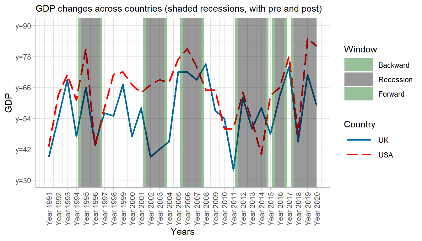

10.3 ggplot Scatter Related Plots

10.3.1 ggplot Scatter Plot

Go back to fan’s REconTools research support package, R4Econ examples page, PkgTestR packaging guide, or Stat4Econ course page.

10.3.1.1 Scatter Plot with Unique Shape, Color, and Label for Each

1. y-axis: horsepower
2. x-axis: time for 1/4 Miles (QSEC)
3. filter: select to display six cars as six scattered points

First, select the relevant variables and filter.

# Include row-name (car-names) as a variable
tb_carnames <- rownames_to_column(mtcars, var = "car_name")  %>% as_tibble()
# Select only six observations for scatter plot
set.seed(789)
it_cars_select <- 8
tb_carnames_selected <- tb_carnames[sample(dim(tb_carnames)[1], it_cars_select, replace=FALSE), ]
# Select only car name and a few variables
tb_carnames_selected <- tb_carnames_selected %>% 
  select(car_name, hp, qsec) %>%
  mutate(car_name = factor(car_name))

Second, add styling for each point:

# https://www.rgbtohex.net/
# https://fanwangecon.github.io/M4Econ/graph/tools/htmlpdfm/fs_color.html
# ar_st_colours <- c(
#   "#262626", "#922428", 
#   "#6b4c9a", "#535154", 
#   "#3e9651", "#396ab1", 
#   "#cc2529", "#ED8137")
ar_st_colours <- c(
  "#922428", "#922428", 
  "#3e9651", "#3e9651", 
  "#396ab1", "#396ab1", 
  "#cc2529", "#cc2529")
# http://sape.inf.usi.ch/quick-reference/ggplot2/shape
# 32 is invisible shape
# ar_it_shapes <- c(32, 5, 17, 15, 1)
ar_it_shapes <- c(
  0, 15, # square
  1, 16, # circle
  2, 17, # triangle
  5, 18 # diamond
  )

Third, draw a scatter plot, with defaults.

# Labeling
st_title <- paste0('Scatter plot of HP and QSEC with unique color and shapes')
st_subtitle <- paste0('https://fanwangecon.github.io/',
                      'R4Econ/tabgraph/ggscatter/htmlpdfr/fs_ggscatter_3cts_mdisc.html')
st_caption <- paste0('mtcars dataset, ',
                     'https://fanwangecon.github.io/R4Econ/')
st_x_label <- 'HP = Horse Power'
st_y_label <- 'QSEC = time for 1/4 Miles'
# Graphing
plt_mtcars_scatter <- tb_carnames_selected %>%
  ggplot(aes(x=hp, y=qsec, 
             colour = car_name, shape = car_name, 
             label=car_name)) +
  geom_point(size=3, stroke = 1.75) + 
  labs(title = st_title, subtitle = st_subtitle,
       x = st_x_label, y = st_y_label, caption = st_caption)
  # geom_text(color='black', size = 3.5, check_overlap = TRUE)
# Display preliminary
# print(plt_mtcars_scatter)

Fourth, add in color and shape for each point based on our specifications.

plt_mtcars_scatter <- plt_mtcars_scatter +    
  scale_colour_manual(values = ar_st_colours) +
  scale_shape_manual(values = ar_it_shapes)
# Display preliminary
print(plt_mtcars_scatter)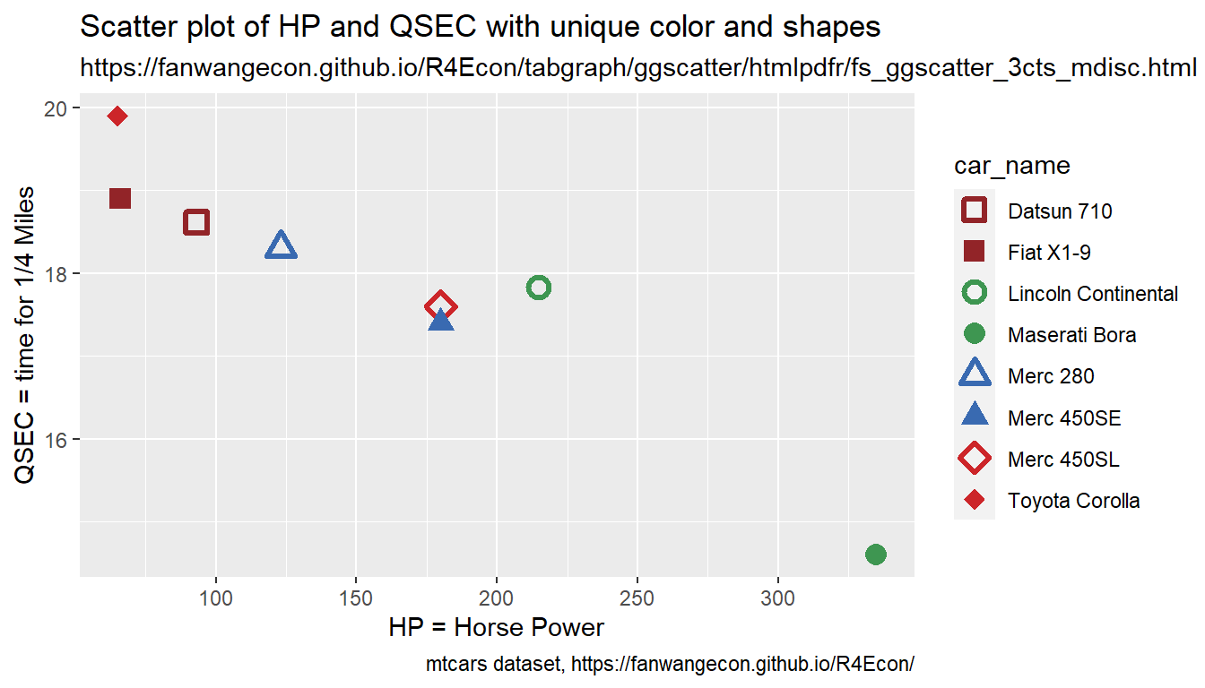

Fifth, axis control, add-in mid-lines and additional layer of axis to show differences from added mid-lines. Add two layers of y and x labels, so that we have levels as well as deviations from the horizontal and vertical lines. Have two layers of labels so that have levels and deviations from levels.

# A. Y-line and X-line
fl_y_line_val <- 18
fl_x_line_val <- 150

# B. X labels
x_breaks <- c(50, 100, 150, 200, 250, 300, 350)
# x labels layer 2
x_breaks_devi <- x_breaks - fl_x_line_val
st_x_breaks_devi <- paste0(x_breaks_devi)
st_x_breaks_devi[x_breaks_devi>0] <- paste0("+", st_x_breaks_devi[x_breaks_devi>0])
st_x_breaks_devi[x_breaks_devi==0] <- paste0("±", st_x_breaks_devi[x_breaks_devi==0])
# x labels layer 1 and 2 joined
x_labels <- paste0(st_x_breaks_devi[1:length(x_breaks)], '\n', x_breaks[1:length(x_breaks)])
# x-bounds
x_min <- 50
x_max <- 350

# C. Y labels layer 1
y_breaks <- seq(14, 20, by=1)
# Y labels layer 2
y_breaks_devi <- y_breaks - fl_y_line_val
st_y_breaks_devi <- paste0(y_breaks_devi)
st_y_breaks_devi[y_breaks_devi>0] <- paste0("+", st_y_breaks_devi[y_breaks_devi>0])
st_y_breaks_devi[y_breaks_devi==0] <- paste0("±", st_y_breaks_devi[y_breaks_devi==0])
# Y labels layer 1 and 2 joined
y_labels <- paste0(y_breaks[1:length(y_breaks)], '\n', st_y_breaks_devi[1:length(y_breaks)])
# y-bounds
y_min <- 14
y_max <- 20

# D. Add custom axis
plt_mtcars_scatter <- plt_mtcars_scatter + 
  geom_hline(yintercept=fl_y_line_val, linetype="dashed", color="black", size=1) + 
  geom_vline(xintercept=fl_x_line_val, linetype="dashed", color="black", size=1) + 
  scale_x_continuous(
    labels = x_labels, breaks = x_breaks,
    limits = c(x_min, x_max)
  ) +
  scale_y_continuous(
    labels = y_labels, breaks = y_breaks,
    limits = c(y_min, y_max)
  )

# E. Rotate Text
plt_mtcars_scatter <- plt_mtcars_scatter + 
  theme(axis.text.y = element_text(angle = 90, hjust = 0.5, vjust = 0.5))

# F. print
print(plt_mtcars_scatter)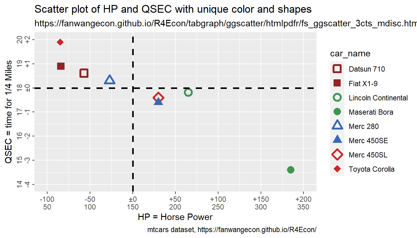

10.3.1.2 Three Continuous Variables and Two Categorical Variables

We will generate a graph that is very similar to the graph shown for fs_tib_factors, with the addition that scatter color and shape will be for two separate variables, and with the addition that scatter size will be for an additional continuous variable.

We have three continuous variables:

1. y-axis: time for 1/4 Miles (QSEC)
2. x-axis: horsepower
3. scatter-size: miles per gallon (mpg)

We have two categorical ariables:

1. color: vs engine shape (vshaped or straight)
2. shape: am shift type (auto or manual)

First, Load in the mtcars dataset and convert to categorical variables to factor with labels.

# First make sure these are factors
tb_mtcars <- as_tibble(mtcars) %>%
  mutate(vs = as_factor(vs), am = as_factor(am))
# Second Label the Factors
am_levels <- c(auto_shift = "0", manual_shift = "1")
vs_levels <- c(vshaped_engine = "0", straight_engine = "1")
tb_mtcars <- tb_mtcars %>%
  mutate(vs = fct_recode(vs, !!!vs_levels),
         am = fct_recode(am, !!!am_levels))

Second, generate the core graph, a scatterplot with a nonlinear trendline. Note that in the example below color and shpae only apply to the jitter scatter, but not the trendline graph.

# Graphing
plt_mtcars_scatter <-
  ggplot(tb_mtcars, aes(x=hp, y=qsec)) +
  geom_jitter(aes(size=mpg, colour=vs, shape=am), width = 0.15) +
  geom_smooth(span = 0.50, se=FALSE) +
  theme_bw()

Third, control Color and Shape Information. There will be two colors and two shapes. See all shape listing.

# Color controls
ar_st_colors <- c("#33cc33", "#F8766D")
ar_st_colors_label <- c("v-shaped", "straight")
fl_legend_color_symbol_size <- 5
st_leg_color_lab <- "Engine-Shape"
# Shape controls
ar_it_shapes <- c(9, 15)
ar_st_shapes_label <- c("auto", "manuel")
fl_legend_shape_symbol_size <- 5
st_leg_shape_lab <- "Transmission"

Fourth, control the size of the scatter, which will be the MPG variable.

# Control scatter point size
fl_min_size <- 3
fl_max_size <- 6
ar_size_range <- c(fl_min_size, fl_max_size)
st_leg_size_lab <- "MPG"

Fifth, control graph strings.

# Labeling
st_title <- paste0('Distribution of HP and QSEC from mtcars')
st_subtitle <- paste0('https://fanwangecon.github.io/',
                      'R4Econ/tabgraph/ggscatter/htmlpdfr/fs_ggscatter_3cts_mdisc.html')
st_caption <- paste0('mtcars dataset, ',
                     'https://fanwangecon.github.io/R4Econ/')
st_x_label <- 'HP = Horse Power'
st_y_label <- 'QSEC = time for 1/4 Miles'

Sixth, combine graphical components.

# Add titles and labels
plt_mtcars_scatter <- plt_mtcars_scatter +
  labs(title = st_title, subtitle = st_subtitle,
       x = st_x_label, y = st_y_label, caption = st_caption)
# Color, shape and size controls
plt_mtcars_scatter <- plt_mtcars_scatter +
  scale_colour_manual(values=ar_st_colors, labels=ar_st_colors_label) +
  scale_shape_manual(values=ar_it_shapes, labels=ar_st_shapes_label) +
  scale_size_continuous(range = ar_size_range)

Eigth, replace default legends titles for color, shape and size.

# replace the default labels for each legend segment
plt_mtcars_scatter <- plt_mtcars_scatter +
  labs(colour = st_leg_color_lab,
       shape = st_leg_shape_lab,
       size = st_leg_size_lab)

Ninth, additional controls for the graph.

# Control the order of legend display
# Show color, show shape, then show size.
plt_mtcars_scatter <- plt_mtcars_scatter + guides(
  colour = guide_legend(order = 1, override.aes = list(size = fl_legend_color_symbol_size)),
  shape = guide_legend(order = 2, override.aes = list(size = fl_legend_shape_symbol_size)),
  size = guide_legend(order = 3))
# show
print(plt_mtcars_scatter)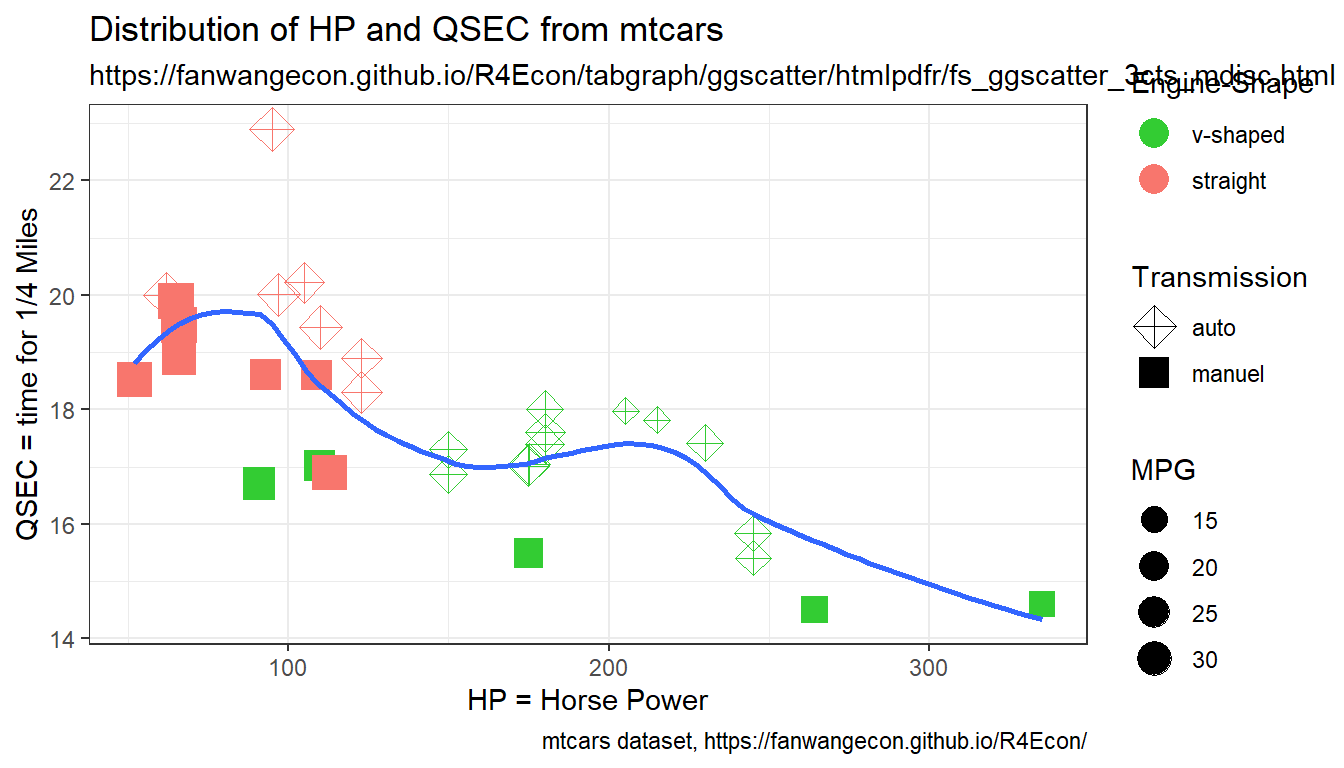

10.3.2 ggplot Multiple Scatter-Lines with Facet Wrap

Go back to fan’s REconTools research support package, R4Econ examples page, PkgTestR packaging guide, or Stat4Econ course page.

10.3.2.1 Multiple Scatter-Lines with Facet Wrap

Two subplots, for auto and manual transitions. The x-axis is horse-power, the y-axis shows QSEC. Different colors represent v-shaped and straight-engines.

1. y-axis: time for 1/4 Miles (QSEC)
2. x-axis: horsepower (hp)
3. facet-wrap: auto or manual (am)
4. colored line and point shapes: vshaped or straight engine (vs)

First, Load in the mtcars dataset and convert to categorical variables to factor with labels.

# First make sure these are factors
tb_mtcars <- as_tibble(mtcars) %>%
  mutate(vs = as_factor(vs), am = as_factor(am))
# Second Label the Factors
am_levels <- c(auto_shift = "0", manual_shift = "1")
vs_levels <- c("vshaped engine" = "0", "straight engine" = "1")
tb_mtcars <- tb_mtcars %>%
  mutate(vs = fct_recode(vs, !!!vs_levels),
         am = fct_recode(am, !!!am_levels))

Second, generate the core graph, a line plot and facet wrapping over the am variable. Note that vs variable has different color as well as line type and shape

# Graphing
plt_mtcars_scatter <-
  ggplot(tb_mtcars, aes(x=hp, y=qsec,
                        colour=am, shape=am, linetype=am)) +
  geom_smooth(se = FALSE, lwd = 1.5) + # Lwd = line width
  geom_point(size = 5, stroke = 2) + # stroke = point shape width
  facet_wrap(~ vs,
             scales = "free_x",
             nrow = 1, ncol = 2,
             labeller = label_wrap_gen(multi_line=FALSE))

Third, control Color, Shape and Line-type Information. There will be two colors, two shapes and two linetypes. See all shape listing and linetype listing., See all shape listing.

# Color controls
ar_st_colors <- c("#33cc33", "#F8766D")
ar_st_colors_label <- c("auto", "manual")
fl_legend_color_symbol_size <- 5
st_leg_color_lab <- "Transmission"
# Shape controls
ar_it_shapes <- c(1, 5)
ar_st_shapes_label <- c("auto", "manual")
fl_legend_shape_symbol_size <- 5
st_leg_shape_lab <- "Transmission"
# Line-Type controls
ar_st_linetypes <- c('solid', 'dashed')
ar_st_linetypes_label <- c("auto", "manual")
fl_legend_linetype_symbol_size <- 5
st_leg_linetype_lab <- "Transmission"

Fourth, manaully specify an x-axis.

# x labeling and axis control
ar_st_x_labels <- c('50 hp', '150 hp', '250 hp', '350 hp')
ar_fl_x_breaks <- c(50, 150, 250, 350)
ar_fl_x_limits <- c(40, 360)
# y labeling and axis control
ar_st_y_labels <- c('15 QSEC', '18', '21', '24 QSEC')
ar_fl_y_breaks <- c(15, 18, 21, 24)
ar_fl_y_limits <- c(13.5, 25.5)

Fifth, control graph strings.

# Labeling
st_title <- paste0('How QSEC varies by Horse-power, by Engine and Transmission Types')
st_subtitle <- paste0('https://fanwangecon.github.io/',
                      'R4Econ/tabgraph/multiplot/htmlpdfr/fs_ggscatter_facet_wrap.html')
st_caption <- paste0('mtcars dataset, ',
                     'https://fanwangecon.github.io/R4Econ/')
st_x_label <- 'HP = Horse Power'
st_y_label <- 'QSEC = time for 1/4 Miles'

Sixth, combine graphical components.

# Add titles and labels
plt_mtcars_scatter <- plt_mtcars_scatter +
  labs(title = st_title, subtitle = st_subtitle,
       x = st_x_label, y = st_y_label, caption = st_caption)

# x and y-axis ticks controls
plt_mtcars_scatter <- plt_mtcars_scatter +
  scale_x_continuous(labels = ar_st_x_labels,
                     breaks = ar_fl_x_breaks,
                     limits = ar_fl_x_limits) +
  scale_y_continuous(labels = ar_st_y_labels,
                     breaks = ar_fl_y_breaks,
                     limits = ar_fl_y_limits)

# Color, shape and linetype controls
plt_mtcars_scatter <- plt_mtcars_scatter +
  scale_colour_manual(values=ar_st_colors, labels=ar_st_colors_label) +
  scale_shape_manual(values=ar_it_shapes, labels=ar_st_shapes_label) +
  scale_linetype_manual(values=ar_st_linetypes, labels=ar_st_linetypes_label)

Seventh, replace default legends, and set figure font overall etc.

# has legend theme
theme_custom <- theme(
  text = element_text(size = 11),
  axis.text.y = element_text(angle = 90),
  legend.title = element_blank(),
  legend.position = c(0.35, 0.80),
  legend.key.width = unit(5, "line"),
  legend.background =
    element_rect(fill = "transparent", colour = "black", linetype='solid'))
# no legend theme (no y)
theme_custom_blank <- theme(
  text = element_text(size = 12),
  legend.title = element_blank(),
  legend.position = "none",
  axis.title.y=element_blank(),
  axis.text.y=element_blank(),
  axis.ticks.y=element_blank())

Eighth, graph out.

# replace the default labels for each legend segment
plt_mtcars_scatter <- plt_mtcars_scatter + theme_custom
# show
print(plt_mtcars_scatter)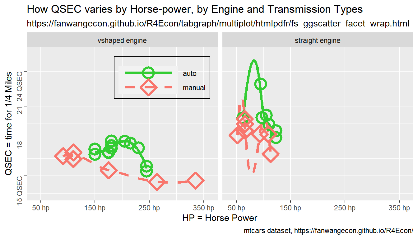

10.3.2.2 Divide Facet Wrapped Plot into Subplots

Given the facet-wrapped plot just generated, now save alternative plot versions, where each subplot is saved by itself. Will simply use the code from above, but call inside lapply over different am categories.

Below generate a matrix with multiple data columns, then use apply over each row of the matrix and select different columns of values for each subplot generation.

First generate with legend versions, then without legend versions. These are versions that would be used to more freely compose graph together.

for (it_subplot_as_own_vsr in c(1,2)) {

  if (it_subplot_as_own_vsr == 1) {
    theme_custom_use <- theme_custom
    # st_file_suffix <- '_haslegend'
    # it_width <- 100
  } else if (it_subplot_as_own_vsr == 2) {
    theme_custom_use <- theme_custom_blank
    # st_file_suffix <- '_nolegend'
    # it_width <- 88
  }

  # unique vs as matrix
  # ar_uniques <-sort(unique(tb_mtcars$vs))
  # mt_unique_vs <- matrix(data=ar_uniques, nrow=length(ar_uniques), ncol=1)
  mt_unique_vs <- tb_mtcars %>% group_by(vs) %>%
    summarize(mpg=mean(mpg)) %>% ungroup()
  # apply over
  ls_plots <- apply(mt_unique_vs, 1, function(ar_vs_cate_row) {
    # 1. Graph main
    plt_mtcars_scatter <-
      ggplot(tb_mtcars %>% filter(vs == ar_vs_cate_row[1]),
             aes(x=hp, y=qsec,
                 colour=am, shape=am, linetype=am)) +
      geom_smooth(se = FALSE, lwd = 1.5) + # Lwd = line width
      geom_point(size = 5, stroke = 2)

    # 2. Add titles and labels
    plt_mtcars_scatter <- plt_mtcars_scatter +
      labs(title = st_title, subtitle = st_subtitle,
           x = st_x_label, y = st_y_label, caption = st_caption)

    # 3. x and y ticks
    plt_mtcars_scatter <- plt_mtcars_scatter +
      scale_x_continuous(labels = ar_st_x_labels, breaks = ar_fl_x_breaks, limits = ar_fl_x_limits) +
      scale_y_continuous(labels = ar_st_y_labels, breaks = ar_fl_y_breaks, limits = ar_fl_y_limits)

    # 4. Color, shape and linetype controls
    plt_mtcars_scatter <- plt_mtcars_scatter +
      scale_colour_manual(values=ar_st_colors, labels=ar_st_colors_label) +
      scale_shape_manual(values=ar_it_shapes, labels=ar_st_shapes_label) +
      scale_linetype_manual(values=ar_st_linetypes, labels=ar_st_linetypes_label)

    # 5. replace the default labels for each legend segment
    plt_mtcars_scatter <- plt_mtcars_scatter + theme_custom_use
  })
  # show
  print(ls_plots)
}

## [[1]]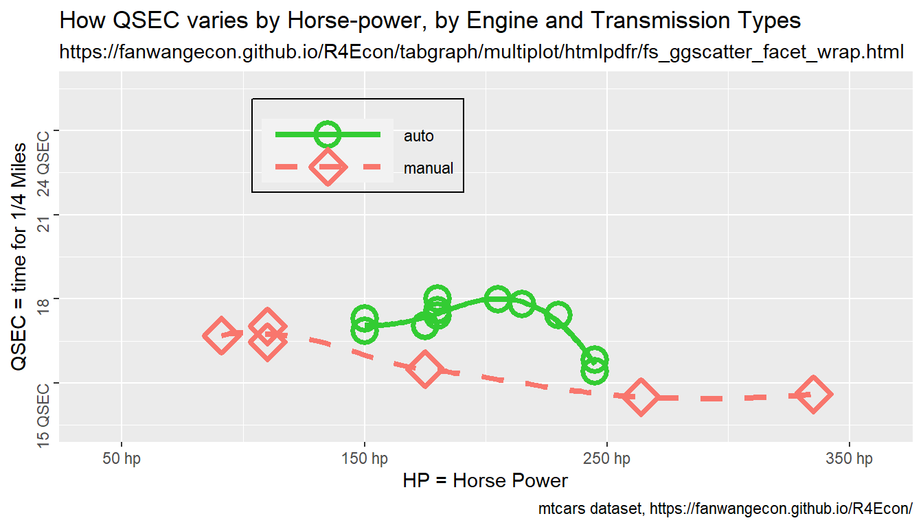

## 
## [[2]]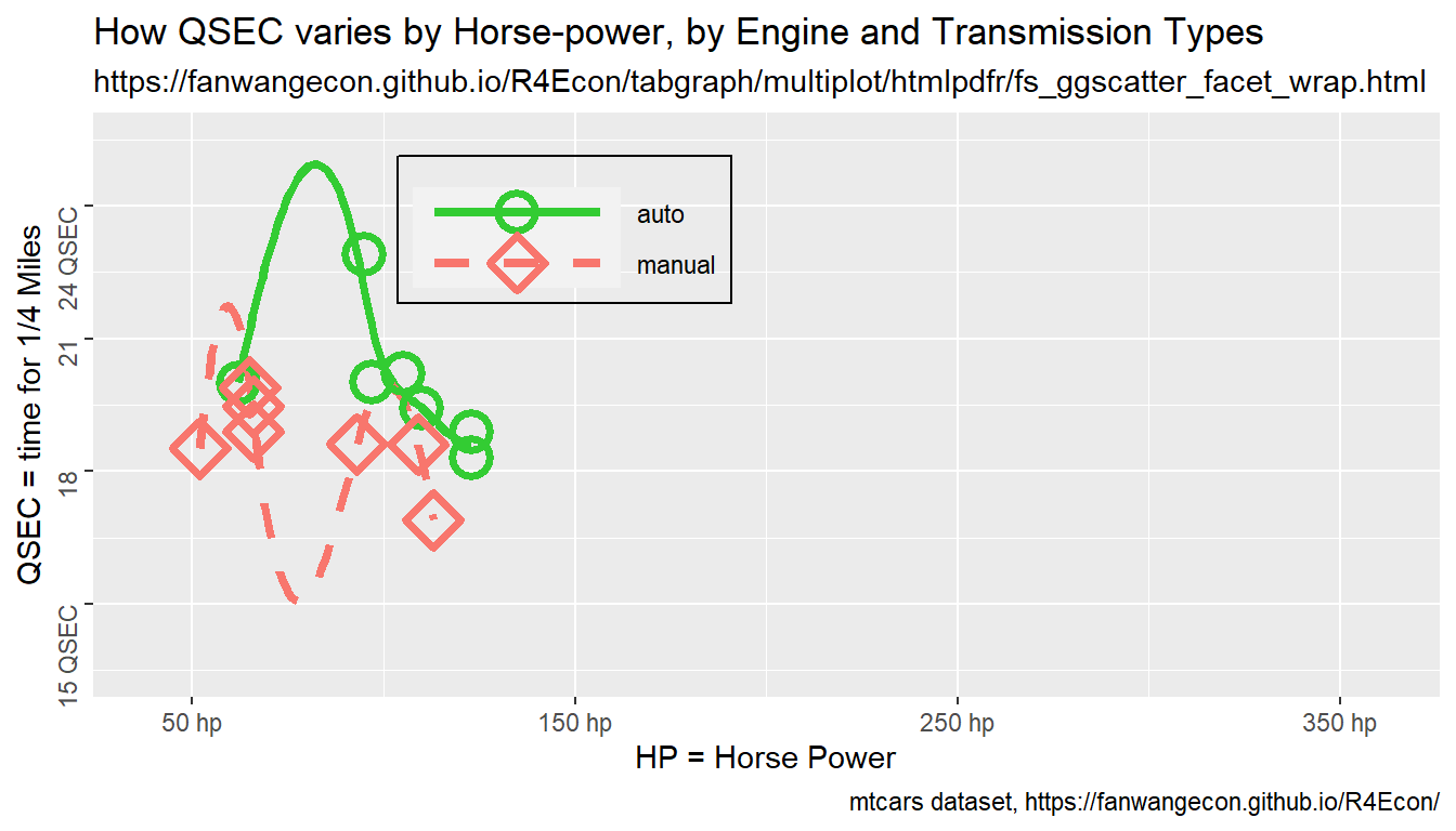

## 
## [[1]]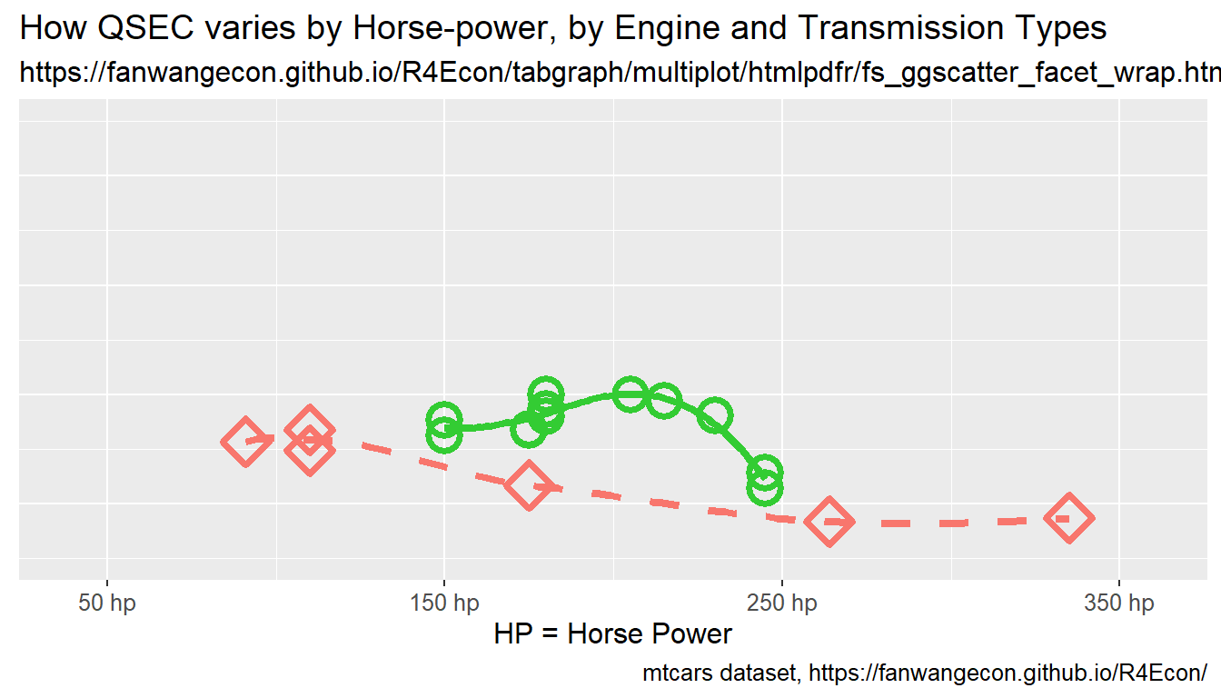

## 
## [[2]]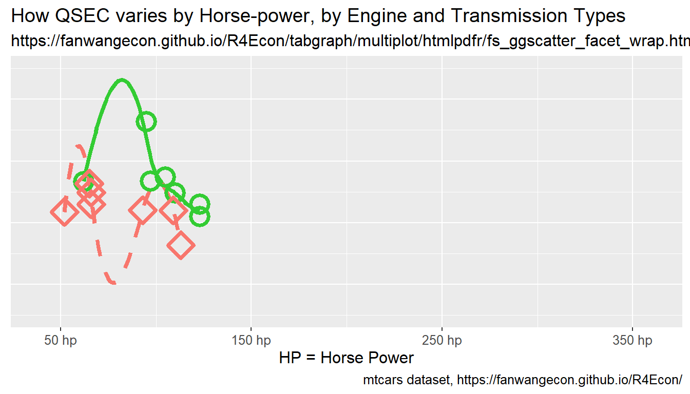

10.4 Write and Read Plots

10.4.1 Import and Export Images

Go back to fan’s REconTools research support package, R4Econ examples page, PkgTestR packaging guide, or Stat4Econ course page.

Work with the R plot function.

10.4.1.1 Export Images Different Formats with Plot()

10.4.1.1.1 Generate and Record A Plot

Generate a graph and recordPlot() it. The generated graph does not have legends Yet. Crucially, there are no titles, legends, axis, labels in the figures. As we stack the figures together, do not add those. Only add at the end jointly for all figure elements together to control at one spot things.

#######################################################
# First, Strings
#######################################################
# Labeling
st_title <- paste0('Scatter, Line and Curve Joint Ploting Example Using Base R\n',
                   'plot() + curve():sin(x)*cos(x), sin(x)+tan(x)+cos(x)')
st_subtitle <- paste0('https://fanwangecon.github.io/',
                      'R4Econ/tabgraph/inout/htmlpdfr/fs_base_curve.html')
st_x_label <- 'x'
st_y_label <- 'f(x)'

#######################################################
# Second, functions
#######################################################
fc_sin_cos_diff <- function(x) sin(x)*cos(x)
st_line_3_y_legend <- 'sin(x)*cos(x)'
fc_sin_cos_tan <- function(x) sin(x) + cos(x) + tan(x)
st_line_4_y_legend <- 'sin(x) + tan(x) + cos(x)'

#######################################################
# Third, patterns
#######################################################
st_line_3_black <- 'black'
st_line_4_purple <- 'orange'
# line type
st_line_3_lty <- 'dotted'
st_line_4_lty <- 'dotdash'
# line width
st_line_3_lwd <- 2.5
st_line_4_lwd <- 3.5

#######################################################
# Fourth: Share xlim and ylim
#######################################################
ar_xlim = c(-3, 3)
ar_ylim = c(-3.5, 3.5)

#######################################################
# Fifth: Even margins
#######################################################
par(new=FALSE)

#######################################################
# Sixth, the four objects and do not print yet:
#######################################################
# Graph Curve 3
par(new=T)
curve(fc_sin_cos_diff,
      col = st_line_3_black,
      lwd = st_line_3_lwd, lty = st_line_3_lty,
      from = ar_xlim[1], to = ar_xlim[2], ylim = ar_ylim,
      ylab = '', xlab = '', yaxt='n', xaxt='n', ann=FALSE)
# Graph Curve 4
par(new=T)
curve(fc_sin_cos_tan,
      col = st_line_4_purple,
      lwd = st_line_4_lwd, lty = st_line_4_lty,
      from = ar_xlim[1], to = ar_xlim[2], ylim = ar_ylim,
      ylab = '', xlab = '', yaxt='n', xaxt='n', ann=FALSE)

pl_curves_save <- recordPlot()

10.4.1.1.2 Generate Large Font and Small Font Versions of PLot

Generate larger font version:

# Replay
pl_curves_save

#######################################################
# Seventh, Set Title and Legend and Plot Jointly
#######################################################
# CEX sizing Contorl Titling and Legend Sizes
fl_ces_fig_reg = 0.75
fl_ces_fig_leg = 0.75
fl_ces_fig_small = 0.65

# R Legend
title(main = st_title, sub = st_subtitle, xlab = st_x_label, ylab = st_y_label,
      cex.lab=fl_ces_fig_reg,
      cex.main=fl_ces_fig_reg,
      cex.sub=fl_ces_fig_small)
axis(1, cex.axis=fl_ces_fig_reg)
axis(2, cex.axis=fl_ces_fig_reg)
grid()

# Legend sizing CEX
legend("topleft",
       bg="transparent",
       bty = "n",
       c(st_line_3_y_legend, st_line_4_y_legend),
       col = c(st_line_3_black, st_line_4_purple),
       pch = c(NA, NA),
       cex = fl_ces_fig_leg,
       lty = c(st_line_3_lty, st_line_4_lty),
       lwd = c(st_line_3_lwd,st_line_4_lwd),
       y.intersp=2)

# record final plot
pl_curves_large <- recordPlot()
dev.off()

Generate smaller font version:

# Replay
pl_curves_save

#######################################################
# Seventh, Set Title and Legend and Plot Jointly
#######################################################
# CEX sizing Contorl Titling and Legend Sizes
fl_ces_fig_reg = 0.45
fl_ces_fig_leg = 0.45
fl_ces_fig_small = 0.25

# R Legend
title(main = st_title, sub = st_subtitle, xlab = st_x_label, ylab = st_y_label,
      cex.lab=fl_ces_fig_reg,
      cex.main=fl_ces_fig_reg,
      cex.sub=fl_ces_fig_small)
axis(1, cex.axis=fl_ces_fig_reg)
axis(2, cex.axis=fl_ces_fig_reg)
grid()

# Legend sizing CEX
legend("topleft",
       bg="transparent",
       bty = "n",
       c(st_line_3_y_legend, st_line_4_y_legend),
       col = c(st_line_3_black, st_line_4_purple),
       pch = c(NA, NA),
       cex = fl_ces_fig_leg,
       lty = c(st_line_3_lty, st_line_4_lty),
       lwd = c(st_line_3_lwd,st_line_4_lwd),
       y.intersp=2)

# record final plot
pl_curves_small <- recordPlot()
dev.off()

10.4.1.1.3 Save Plot with Varying Resolutions and Heights

Export recorded plot.

A4 paper is 8.3 x 11.7, with 1 inch margins, the remaining area is 6.3 x 9.7. For figures that should take half of the page, the height should be 4.8 inch. One third of a page should be 3.2 inch. 6.3 inch is 160mm and 3 inch is 76 mm. In the example below, use

# Store both in within folder directory and root image directory:
# C:\Users\fan\R4Econ\tabgraph\inout\_img
# C:\Users\fan\R4Econ\_img
# need to store in both because bookdown and indi pdf path differ.
# Wrap in try because will not work underbookdown, but images already created

ls_spt_root <- c('..//..//', '')
spt_prefix <- '_img/fs_img_io_2curve'

for (spt_root in ls_spt_root) {
  # Changing pointsize will not change font sizes inside, just rescale
  # PNG 72
  try(png(paste0(spt_root, spt_prefix, "_w135h76_res72.png"),
      width = 135 , height = 76, units='mm', res = 72, pointsize=7))
  print(pl_curves_large)
  dev.off()
  # PNG 300
  try(png(paste0(spt_root, spt_prefix, "_w135h76_res300.png"),
      width = 135, height = 76, units='mm', res = 300, pointsize=7))
  print(pl_curves_large)
  dev.off()
  # PNG 300, SMALL, POINT SIZE LOWER
  try(png(paste0(spt_root, spt_prefix, "_w80h48_res300.png"),
      width = 80, height = 48, units='mm', res = 300, pointsize=7))
  print(pl_curves_small)
  dev.off()
  # PNG 300
  try(png(paste0(spt_root, spt_prefix, "_w160h100_res300.png"),
      width = 160, height = 100, units='mm', res = 300))
  print(pl_curves_large)
  dev.off()

  # EPS
  setEPS()
  try(postscript(paste0(spt_root, spt_prefix, "_fs_2curve.eps")))
  print(pl_curves_large)
  dev.off()
}

## Error in png(paste0(spt_root, spt_prefix, "_w135h76_res72.png"), width = 135,  : 
##   unable to start png() device
## Error in png(paste0(spt_root, spt_prefix, "_w135h76_res300.png"), width = 135,  : 
##   unable to start png() device
## Error in png(paste0(spt_root, spt_prefix, "_w80h48_res300.png"), width = 80,  : 
##   unable to start png() device
## Error in png(paste0(spt_root, spt_prefix, "_w160h100_res300.png"), width = 160,  : 
##   unable to start png() device
## Error in postscript(paste0(spt_root, spt_prefix, "_fs_2curve.eps")) : 
##   cannot open file '..//..//_img/fs_img_io_2curve_fs_2curve.eps'

10.4.1.1.4 Low and High Resolution Figure

The standard resolution often produces very low quality images. Resolution should be increased. See figure comparison.

10.4.1.1.5 Smaller and Larger Figures

Smaller and larger figures with different font size comparison. Note that earlier, we generated the figure without legends, labels, etc first, recorded the figure. Then we associated the same underlying figure with differently sized titles, legends, axis, labels.